Skip to content

Data Quality for Machine Learning


An illustrative look at the importance of data quality in machine learning.
Goku Mohandas
Goku Mohandas
· · ·
Repository Β· Notebook

Subscribe to our newsletter

πŸ“¬  Receive new lessons straight to your inbox (once a month) and join 40K+ developers in learning how to responsibly deliver value with ML.


Overview

In a nutshell, a machine learning model consumes input data and produces predictions. The quality of the predictions directly corresponds to the quality of data you train the model with; garbage in, garbage out. Check out this article on where it makes sense to use AI and how to properly apply it.

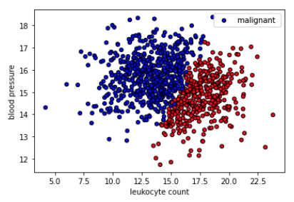
We're going to go through all the concepts with concrete code examples and some synthesized data to train our models on. The task is to determine whether a tumor will be benign (harmless) or malignant (harmful) based on leukocyte (white blood cells) count and blood pressure. This is a synthetic dataset that we created and has no clinical relevance.

Set up

We'll set our seeds for reproducibility.

1
2
import numpy as np
import random
1
SEED = 1234
1
2
3
# Set seed for reproducibility
np.random.seed(SEED)
random.seed(SEED)

Full dataset

We'll first train a model with the entire dataset. Later we'll remove a subset of the dataset and see the effect it has on our model.

Load data

1
2
3
import matplotlib.pyplot as plt
import pandas as pd
from pandas.plotting import scatter_matrix
1
2
3
4
5
# Load data
url = "https://raw.githubusercontent.com/GokuMohandas/Made-With-ML/main/datasets/tumors.csv"
df = pd.read_csv(url, header=0) # load
df = df.sample(frac=1).reset_index(drop=True) # shuffle
df.head()

leukocyte_count blood_pressure tumor_class
0 15.335860 14.637535 benign
1 9.857535 14.518942 malignant
2 17.632579 15.869585 benign
3 18.369174 14.774547 benign
4 14.509367 15.892224 malignant
1
2
3
4
5
# Define X and y
X = df[["leukocyte_count", "blood_pressure"]].values
y = df["tumor_class"].values
print ("X: ", np.shape(X))
print ("y: ", np.shape(y))
X:  (1000, 2)
y:  (1000,)
1
2
3
4
5
6
7
# Plot data
colors = {"benign": "red", "malignant": "blue"}
plt.scatter(X[:, 0], X[:, 1], c=[colors[_y] for _y in y], s=25, edgecolors="k")
plt.xlabel("leukocyte count")
plt.ylabel("blood pressure")
plt.legend(["malignant", "benign"], loc="upper right")
plt.show()
multi-class dataset

We want to choose features that have strong predictive signal for our task. If you want to improve performance, you need to continuously do feature engineering by collecting and adding new signals. So you may run into a new feature that has high correlation (orthogonal signal) with your existing features but it may still possess some unique signal to boost your predictive performance.

1
2
3
# Correlation matrix
scatter_matrix(df, figsize=(5, 5));
df.corr()

leukocyte_count blood_pressure
leukocyte_count 1.000000 -0.162875
blood_pressure -0.162875 1.000000
correlation

Split data

1
2
import collections
from sklearn.model_selection import train_test_split
1
2
3
TRAIN_SIZE = 0.70
VAL_SIZE = 0.15
TEST_SIZE = 0.15
1
2
3
4
5
def train_val_test_split(X, y, train_size):
    """Split dataset into data splits."""
    X_train, X_, y_train, y_ = train_test_split(X, y, train_size=TRAIN_SIZE, stratify=y)
    X_val, X_test, y_val, y_test = train_test_split(X_, y_, train_size=0.5, stratify=y_)
    return X_train, X_val, X_test, y_train, y_val, y_test
1
2
3
4
5
6
7
# Create data splits
X_train, X_val, X_test, y_train, y_val, y_test = train_val_test_split(
    X=X, y=y, train_size=TRAIN_SIZE)
print (f"X_train: {X_train.shape}, y_train: {y_train.shape}")
print (f"X_val: {X_val.shape}, y_val: {y_val.shape}")
print (f"X_test: {X_test.shape}, y_test: {y_test.shape}")
print (f"Sample point: {X_train[0]} β†’ {y_train[0]}")

X_train: (700, 2), y_train: (700,)
X_val: (150, 2), y_val: (150,)
X_test: (150, 2), y_test: (150,)
Sample point: [11.5066204  15.98030799] β†’ malignant

Label encoding

1
from sklearn.preprocessing import LabelEncoder
1
2
# Output vectorizer
label_encoder = LabelEncoder()
1
2
3
4
# Fit on train data
label_encoder = label_encoder.fit(y_train)
classes = list(label_encoder.classes_)
print (f"classes: {classes}")

classes: ["benign", "malignant"]
1
2
3
4
5
6
# Convert labels to tokens
print (f"y_train[0]: {y_train[0]}")
y_train = label_encoder.transform(y_train)
y_val = label_encoder.transform(y_val)
y_test = label_encoder.transform(y_test)
print (f"y_train[0]: {y_train[0]}")
y_train[0]: malignant
y_train[0]: 1
1
2
3
4
# Class weights
counts = np.bincount(y_train)
class_weights = {i: 1.0/count for i, count in enumerate(counts)}
print (f"counts: {counts}\nweights: {class_weights}")
counts: [272 428]
weights: {0: 0.003676470588235294, 1: 0.002336448598130841}

Standardize data

1
from sklearn.preprocessing import StandardScaler
1
2
# Standardize the data (mean=0, std=1) using training data
X_scaler = StandardScaler().fit(X_train)
1
2
3
4
# Apply scaler on training and test data (don't standardize outputs for classification)
X_train = X_scaler.transform(X_train)
X_val = X_scaler.transform(X_val)
X_test = X_scaler.transform(X_test)
1
2
3
# Check (means should be ~0 and std should be ~1)
print (f"X_test[0]: mean: {np.mean(X_test[:, 0], axis=0):.1f}, std: {np.std(X_test[:, 0], axis=0):.1f}")
print (f"X_test[1]: mean: {np.mean(X_test[:, 1], axis=0):.1f}, std: {np.std(X_test[:, 1], axis=0):.1f}")

X_test[0]: mean: 0.0, std: 1.0
X_test[1]: mean: 0.0, std: 1.0

Model

1
2
3
import torch
from torch import nn
import torch.nn.functional as F
1
2
# Set seed for reproducibility
torch.manual_seed(SEED)
1
2
3
INPUT_DIM = 2 # X is 2-dimensional
HIDDEN_DIM = 100
NUM_CLASSES = 2
 1
 2
 3
 4
 5
 6
 7
 8
 9
10
class MLP(nn.Module):
    def __init__(self, input_dim, hidden_dim, num_classes):
        super(MLP, self).__init__()
        self.fc1 = nn.Linear(input_dim, hidden_dim)
        self.fc2 = nn.Linear(hidden_dim, num_classes)

    def forward(self, x_in):
        z = F.relu(self.fc1(x_in)) # ReLU activation function added!
        z = self.fc2(z)
        return z
1
2
3
# Initialize model
model = MLP(input_dim=INPUT_DIM, hidden_dim=HIDDEN_DIM, num_classes=NUM_CLASSES)
print (model.named_parameters)

<bound method Module.named_parameters of MLP(
  (fc1): Linear(in_features=2, out_features=100, bias=True)
  (fc2): Linear(in_features=100, out_features=2, bias=True)
)>

Training

1
from torch.optim import Adam
1
2
3
LEARNING_RATE = 1e-3
NUM_EPOCHS = 5
BATCH_SIZE = 32
1
2
3
# Define Loss
class_weights_tensor = torch.Tensor(list(class_weights.values()))
loss_fn = nn.CrossEntropyLoss(weight=class_weights_tensor)
1
2
3
4
5
# Accuracy
def accuracy_fn(y_pred, y_true):
    n_correct = torch.eq(y_pred, y_true).sum().item()
    accuracy = (n_correct / len(y_pred)) * 100
    return accuracy
1
2
# Optimizer
optimizer = Adam(model.parameters(), lr=LEARNING_RATE)
1
2
3
4
5
6
7
# Convert data to tensors
X_train = torch.Tensor(X_train)
y_train = torch.LongTensor(y_train)
X_val = torch.Tensor(X_val)
y_val = torch.LongTensor(y_val)
X_test = torch.Tensor(X_test)
y_test = torch.LongTensor(y_test)
 1
 2
 3
 4
 5
 6
 7
 8
 9
10
11
12
13
14
15
16
17
18
19
20
21
# Training
for epoch in range(NUM_EPOCHS*10):
    # Forward pass
    y_pred = model(X_train)

    # Loss
    loss = loss_fn(y_pred, y_train)

    # Zero all gradients
    optimizer.zero_grad()

    # Backward pass
    loss.backward()

    # Update weights
    optimizer.step()

    if epoch%10==0:
        predictions = y_pred.max(dim=1)[1] # class
        accuracy = accuracy_fn(y_pred=predictions, y_true=y_train)
        print (f"Epoch: {epoch} | loss: {loss:.2f}, accuracy: {accuracy:.1f}")

Epoch: 0 | loss: 0.70, accuracy: 49.6
Epoch: 10 | loss: 0.54, accuracy: 93.7
Epoch: 20 | loss: 0.43, accuracy: 97.1
Epoch: 30 | loss: 0.35, accuracy: 97.0
Epoch: 40 | loss: 0.30, accuracy: 97.4

Evaluation

1
2
3
import json
import matplotlib.pyplot as plt
from sklearn.metrics import precision_recall_fscore_support
 1
 2
 3
 4
 5
 6
 7
 8
 9
10
11
12
13
14
15
16
17
18
19
20
21
22
23
def get_metrics(y_true, y_pred, classes):
    """Per-class performance metrics."""
    # Performance
    performance = {"overall": {}, "class": {}}

    # Overall performance
    metrics = precision_recall_fscore_support(y_true, y_pred, average="weighted")
    performance["overall"]["precision"] = metrics[0]
    performance["overall"]["recall"] = metrics[1]
    performance["overall"]["f1"] = metrics[2]
    performance["overall"]["num_samples"] = np.float64(len(y_true))

    # Per-class performance
    metrics = precision_recall_fscore_support(y_true, y_pred, average=None)
    for i in range(len(classes)):
        performance["class"][classes[i]] = {
            "precision": metrics[0][i],
            "recall": metrics[1][i],
            "f1": metrics[2][i],
            "num_samples": np.float64(metrics[3][i]),
        }

    return performance
1
2
3
# Predictions
y_prob = F.softmax(model(X_test), dim=1)
y_pred = y_prob.max(dim=1)[1]
1
2
3
# # Performance
performance = get_metrics(y_true=y_test, y_pred=y_pred, classes=classes)
print (json.dumps(performance, indent=2))

{
  "overall": {
    "precision": 0.9461538461538461,
    "recall": 0.9619565217391304,
    "f1": 0.9517707041477195,
    "num_samples": 150.0
  },
  "class": {
    "benign": {
      "precision": 0.8923076923076924,
      "recall": 1.0,
      "f1": 0.9430894308943091,
      "num_samples": 58.0
    },
    "malignant": {
      "precision": 1.0,
      "recall": 0.9239130434782609,
      "f1": 0.96045197740113,
      "num_samples": 92.0
    }
  }
}

Inference

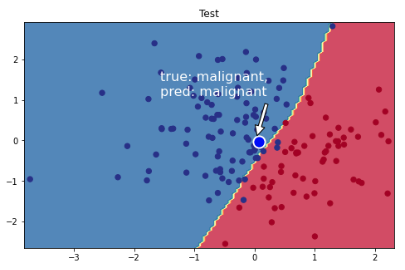
We're going to plot a point, which we know belongs to the malignant tumor class. Our well trained model here would accurately predict that it is indeed a malignant tumor!

 1
 2
 3
 4
 5
 6
 7
 8
 9
10
11
12
13
14
def plot_multiclass_decision_boundary(model, X, y):
    x_min, x_max = X[:, 0].min() - 0.1, X[:, 0].max() + 0.1
    y_min, y_max = X[:, 1].min() - 0.1, X[:, 1].max() + 0.1
    xx, yy = np.meshgrid(np.linspace(x_min, x_max, 101), np.linspace(y_min, y_max, 101))
    cmap = plt.cm.Spectral

    X_test = torch.from_numpy(np.c_[xx.ravel(), yy.ravel()]).float()
    y_pred = F.softmax(model(X_test), dim=1)
    _, y_pred = y_pred.max(dim=1)
    y_pred = y_pred.reshape(xx.shape)
    plt.contourf(xx, yy, y_pred, cmap=plt.cm.Spectral, alpha=0.8)
    plt.scatter(X[:, 0], X[:, 1], c=y, s=40, cmap=plt.cm.RdYlBu)
    plt.xlim(xx.min(), xx.max())
    plt.ylim(yy.min(), yy.max())
 1
 2
 3
 4
 5
 6
 7
 8
 9
10
11
12
13
14
15
16
17
18
19
20
# Visualize the decision boundary
plt.figure(figsize=(8,5))
plt.title("Test")
plot_multiclass_decision_boundary(model=model, X=X_test, y=y_test)

# Sample point near the decision boundary
mean_leukocyte_count, mean_blood_pressure = X_scaler.transform(
    [[np.mean(df.leukocyte_count), np.mean(df.blood_pressure)]])[0]
plt.scatter(mean_leukocyte_count+0.05, mean_blood_pressure-0.05, s=200,
            c="b", edgecolor="w", linewidth=2)

# Annotate
plt.annotate("true: malignant,\npred: malignant",
             color="white",
             xy=(mean_leukocyte_count, mean_blood_pressure),
             xytext=(0.4, 0.65),
             textcoords="figure fraction",
             fontsize=16,
             arrowprops=dict(facecolor="white", shrink=0.1))
plt.show()

correct prediction

Great! We received great performances on both our train and test data splits. We're going to use this dataset to show the importance of data quality.
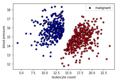
Reduced dataset

Let's remove some training data near the decision boundary and see how robust the model is now.

Load data

1
2
3
4
5
# Raw reduced data
url = "https://raw.githubusercontent.com/GokuMohandas/Made-With-ML/main/datasets/tumors_reduced.csv"
df_reduced = pd.read_csv(url, header=0) # load
df_reduced = df_reduced.sample(frac=1).reset_index(drop=True) # shuffle
df_reduced.head()
leukocyte_count blood_pressure tumor_class
0 16.795186 14.434741 benign
1 13.472969 15.250393 malignant
2 9.840450 16.434717 malignant
3 16.390730 14.419258 benign
4 13.367974 15.741790 malignant
1
2
3
4
5
# Define X and y
X = df_reduced[["leukocyte_count", "blood_pressure"]].values
y = df_reduced["tumor_class"].values
print ("X: ", np.shape(X))
print ("y: ", np.shape(y))
X:  (720, 2)
y:  (720,)
1
2
3
4
5
6
7
# Plot data
colors = {"benign": "red", "malignant": "blue"}
plt.scatter(X[:, 0], X[:, 1], c=[colors[_y] for _y in y], s=25, edgecolors="k")
plt.xlabel("leukocyte count")
plt.ylabel("blood pressure")
plt.legend(["malignant", "benign"], loc="upper right")
plt.show()
reduced dataset

Split data

1
2
3
4
5
6
7
# Create data splits
X_train, X_val, X_test, y_train, y_val, y_test = train_val_test_split(
    X=X, y=y, train_size=TRAIN_SIZE)
print (f"X_train: {X_train.shape}, y_train: {y_train.shape}")
print (f"X_val: {X_val.shape}, y_val: {y_val.shape}")
print (f"X_test: {X_test.shape}, y_test: {y_test.shape}")
print (f"Sample point: {X_train[0]} β†’ {y_train[0]}")
X_train: (503, 2), y_train: (503,)
X_val: (108, 2), y_val: (108,)
X_test: (109, 2), y_test: (109,)
Sample point: [19.66235758 15.65939541] β†’ benign

Label encoding

1
2
3
4
5
6
7
# Encode class labels
label_encoder = LabelEncoder()
label_encoder = label_encoder.fit(y_train)
num_classes = len(label_encoder.classes_)
y_train = label_encoder.transform(y_train)
y_val = label_encoder.transform(y_val)
y_test = label_encoder.transform(y_test)
1
2
3
4
# Class weights
counts = np.bincount(y_train)
class_weights = {i: 1.0/count for i, count in enumerate(counts)}
print (f"counts: {counts}\nweights: {class_weights}")

counts: [272 231]
weights: {0: 0.003676470588235294, 1: 0.004329004329004329}

Standardize data

1
2
3
4
5
# Standardize inputs using training data
X_scaler = StandardScaler().fit(X_train)
X_train = X_scaler.transform(X_train)
X_val = X_scaler.transform(X_val)
X_test = X_scaler.transform(X_test)

Model

1
2
# Initialize model
model = MLP(input_dim=INPUT_DIM, hidden_dim=HIDDEN_DIM, num_classes=NUM_CLASSES)

Training

1
2
3
# Define Loss
class_weights_tensor = torch.Tensor(list(class_weights.values()))
loss_fn = nn.CrossEntropyLoss(weight=class_weights_tensor)
1
2
# Optimizer
optimizer = Adam(model.parameters(), lr=LEARNING_RATE)
1
2
3
4
5
6
7
# Convert data to tensors
X_train = torch.Tensor(X_train)
y_train = torch.LongTensor(y_train)
X_val = torch.Tensor(X_val)
y_val = torch.LongTensor(y_val)
X_test = torch.Tensor(X_test)
y_test = torch.LongTensor(y_test)
 1
 2
 3
 4
 5
 6
 7
 8
 9
10
11
12
13
14
15
16
17
18
19
20
21
# Training
for epoch in range(NUM_EPOCHS*10):
    # Forward pass
    y_pred = model(X_train)

    # Loss
    loss = loss_fn(y_pred, y_train)

    # Zero all gradients
    optimizer.zero_grad()

    # Backward pass
    loss.backward()

    # Update weights
    optimizer.step()

    if epoch%10==0:
        predictions = y_pred.max(dim=1)[1] # class
        accuracy = accuracy_fn(y_pred=predictions, y_true=y_train)
        print (f"Epoch: {epoch} | loss: {loss:.2f}, accuracy: {accuracy:.1f}")

Epoch: 0 | loss: 0.68, accuracy: 69.8
Epoch: 10 | loss: 0.53, accuracy: 99.6
Epoch: 20 | loss: 0.42, accuracy: 99.6
Epoch: 30 | loss: 0.33, accuracy: 99.6
Epoch: 40 | loss: 0.27, accuracy: 99.8

Evaluation

1
2
3
# Predictions
y_prob = F.softmax(model(X_test), dim=1)
y_pred = y_prob.max(dim=1)[1]
1
2
3
# # Performance
performance = get_metrics(y_true=y_test, y_pred=y_pred, classes=classes)
print (json.dumps(performance, indent=2))

{
  "overall": {
    "precision": 1.0,
    "recall": 1.0,
    "f1": 1.0,
    "num_samples": 109.0
  },
  "class": {
    "benign": {
      "precision": 1.0,
      "recall": 1.0,
      "f1": 1.0,
      "num_samples": 59.0
    },
    "malignant": {
      "precision": 1.0,
      "recall": 1.0,
      "f1": 1.0,
      "num_samples": 50.0
    }
  }
}

Inference

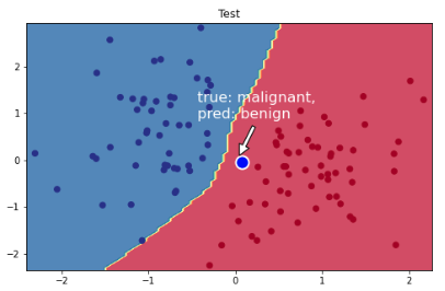
Now let's see how the same inference point from earlier performs now on the model trained on the reduced dataset.

 1
 2
 3
 4
 5
 6
 7
 8
 9
10
11
12
13
14
15
16
17
18
# Visualize the decision boundary
plt.figure(figsize=(8,5))
plt.title("Test")
plot_multiclass_decision_boundary(model=model, X=X_test, y=y_test)

# Sample point near the decision boundary (same point as before)
plt.scatter(mean_leukocyte_count+0.05, mean_blood_pressure-0.05, s=200,
            c="b", edgecolor="w", linewidth=2)

# Annotate
plt.annotate("true: malignant,\npred: benign",
             color="white",
             xy=(mean_leukocyte_count, mean_blood_pressure),
             xytext=(0.45, 0.60),
             textcoords="figure fraction",
             fontsize=16,
             arrowprops=dict(facecolor="white", shrink=0.1))
plt.show()
incorrect prediction

This is a very fragile but highly realistic scenario. Based on our reduced synthetic dataset, we have achieved a model that generalized really well on the test data. But when we ask for the prediction for the same point tested earlier (which we known is malignant), the prediction is now a benign tumor. We would have completely missed the tumor. To mitigate this, we can:

  1. Get more data around the space we are concerned about
  2. Consume predictions with caution when they are close to the decision boundary

Takeaway

Models are not crystal balls. So it's important that before any machine learning, we really look at our data and ask ourselves if it is truly representative for the task we want to solve. The model itself may fit really well and generalize well on your data but if the data is of poor quality to begin with, the model cannot be trusted.

Once you are confident that your data is of good quality, you can finally start thinking about modeling. The type of model you choose depends on many factors, including the task, type of data, complexity required, etc.

So once you figure out what type of model your task needs, start with simple models and then slowly add complexity. You don’t want to start with neural networks right away because that may not be right model for your data and task. Striking this balance in model complexity is one of the key tasks of your data scientists. simple models β†’ complex models


To cite this content, please use:

1
2
3
4
5
6
@article{madewithml,
    author       = {Goku Mohandas},
    title        = { Data quality - Made With ML },
    howpublished = {\url{https://madewithml.com/}},
    year         = {2023}
}