Distributed training
Repository · Notebook

Subscribe to our newsletter
📬 Receive new lessons straight to your inbox (once a month) and join 40K+ developers in learning how to responsibly deliver value with ML.
Intuition
Now that we have our data prepared, we can start training our models to optimize on our objective. Ideally, we would start with the simplest possible baseline and slowly add complexity to our models:
- Start with a random (chance) model.
Since we have four classes, we may expect a random model to be correct around 25% of the time but recall that not all of our classes have equal counts.
- Develop a rule-based approach using if-else statements, regular expressions, etc.
We could build a list of common words for each class and if a word in the input matches a word in the list, we can predict that class.
- Slowly add complexity by addressing limitations and motivating representations and model architectures.
We could start with a simple term frequency (TF-IDF) mode and then move onto embeddings with CNNs, RNNs, Transformers, etc.
- Weigh tradeoffs (performance, latency, size, etc.) between performant baselines.
- Revisit and iterate on baselines as your dataset grows and new model architectures are developed.
We're going to skip straight to step 3 of developing a complex model because this task involves unstructured data and rule-based systems are not well suited for this. And with the increase adoption of large language models (LLMs) as a proven model architecture for NLP tasks, we'll fine-tune a pretrained LLM on our dataset.
Iterate on the data
Instead of using a fixed dataset and iterating on the models, we could keep the model constant and iterate on the dataset. This is useful to improve the quality of our datasets.
- remove or fix data samples (false positives & negatives)
- prepare and transform features
- expand or consolidate classes
- incorporate auxiliary datasets
- identify unique slices to boost
Distributed training
With the rapid increase in data (unstructured) and model sizes (ex. LLMs), it's becoming increasingly difficult to train models on a single machine. We need to be able to distribute our training across multiple machines in order to train our models in a reasonable amount of time. And we want to be able to do this without having to:
- set up a cluster by individually (and painstakingly) provisioning compute resources (CPU, GPU, etc.)
- writing complex code to distribute our training across multiple machines
- worry about communication and resource utilization between our different distributed compute resources
- worry about fault tolerance and recovery from our large training workloads
To address all of these concerns, we'll be using Ray Train here in order to create a training workflow that can scale across multiple machines. While there are many options to choose from for distributed training, such as Pytorch Distributed Data Parallel (DDP), Horovod, etc., none of them allow us to scale across different machines with ease and do so with minimal changes to our single-machine training code as Ray does.
Primer on distributed training
With distributed training, there will be a head node that's responsible for orchestrating the training process. While the worker nodes that will be responsible for training the model and communicating results back to the head node. From a user's perspective, Ray abstracts away all of this complexity and we can simply define our training functionality with minimal changes to our code (as if we were training on a single machine).
Generative AI
In this lesson, we're going to be fine-tuning a pretrained large language model (LLM) using our labeled dataset. The specific class of LLMs we'll be using is called BERT. Bert models are encoder-only models and are the gold-standard for supervised NLP tasks. However, you may be wondering how do all the (much larger) LLM, created for generative applications, fare (GPT 4, Falcon 40B, Llama 2, etc.)?
We chose the smaller BERT model for our course because it's easier to train and fine-tune. However, the workflow for fine-tuning the larger LLMs are quite similar as well. They do require much more compute but Ray abstracts away the scaling complexities involved with that.
Note
All the code for this section can be found in our separate benchmarks.ipynb notebook.
Set up
You'll need to first sign up for an OpenAI account and then grab your API key from here.
1 2 | |
Load data
We'll first load the our training and inference data into dataframes.
1 | |
1 2 3 4 | |
1 2 3 | |
['computer-vision', 'other', 'natural-language-processing', 'mlops']
1 2 3 | |
Utilities
We'll define a few utility functions to make the OpenAI request and to store our predictions. While we could perform batch prediction by loading samples until the context length is reached, we'll just perform one at a time since it's not too many data points and we can have fully deterministic behavior (if you insert new data, etc.). We'll also added some reliability in case we overload the endpoints with too many request at once.
1 2 3 4 5 6 7 | |
We'll first define what a sample call to the OpenAI endpoint looks like. We'll pass in:
- system_content that has information about how the LLM should behave.
- assistant_content for any additional context it should have for answering our questions.
- user_content that has our message or query to the LLM.
- model should specify which specific model we want to send our request to.
We can pass all of this information in through the openai.ChatCompletion.create function to receive our response.
1 2 3 4 5 6 7 8 9 10 11 12 13 | |
I'm doing just fine, so glad you ask,
Rhyming away, up to the task.
How about you, my dear friend?
Tell me how your day did ascend.
Now, let's create a function that can predict tags for a given sample.
1 2 3 4 5 6 7 8 9 10 11 12 13 14 15 16 | |
1 2 3 4 5 6 7 8 9 10 11 | |
natural-language-processing
Next, let's create a function that can predict tags for a list of inputs.
1 2 3 | |
[{'title': 'Diffusion to Vector',
  'description': 'Reference implementation of Diffusion2Vec (Complenet 2018) built on Gensim and NetworkX. '},
 {'title': 'Graph Wavelet Neural Network',
  'description': 'A PyTorch implementation of "Graph Wavelet Neural Network" (ICLR 2019) '},
 {'title': 'Capsule Graph Neural Network',
  'description': 'A PyTorch implementation of "Capsule Graph Neural Network" (ICLR 2019).'}]
1 2 3 4 5 6 7 8 9 10 11 12 13 14 15 16 17 18 19 20 21 22 | |
1 2 | |
100%|██████████| 3/3 [00:01<00:00,  2.96its]
['computer-vision', 'computer-vision', 'computer-vision']
Next we'll define a function that can clean our predictions in the event that it's not the proper format or has hallucinated a tag outside of our expected tags.
1 2 3 4 5 6 7 | |
Tip
Open AI has now released function calling and custom instructions which is worth exploring to avoid this manual cleaning.
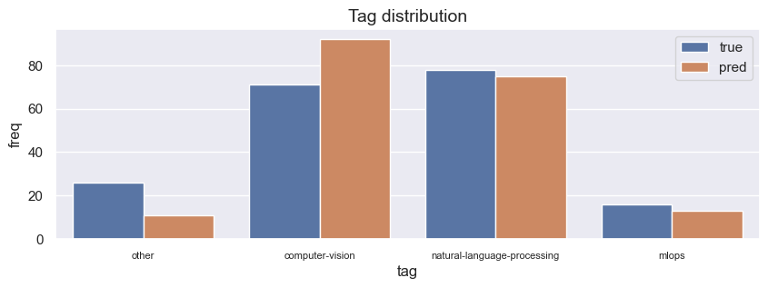
Next, we'll define a function that will plot our ground truth labels and predictions.
1 2 3 4 5 6 7 8 9 10 11 12 13 14 15 | |
And finally, we'll define a function that will combine all the utilities above to predict, clean and plot our results.
1 2 3 4 5 6 7 8 9 10 11 12 13 14 15 | |
Zero-shot learning
Now we're ready to start benchmarking our different LLMs with different context.
1 2 | |
We'll start with zero-shot learning which involves providing the model with the system_content that tells it how to behave but no examples of the behavior (no assistant_content).
1 2 3 4 5 | |
1 2 3 4 5 | |
100%|██████████| 191/191 [11:01<00:00,  3.46s/it]
{
  "precision": 0.7919133278407181,
  "recall": 0.806282722513089,
  "f1": 0.7807530967691199
}
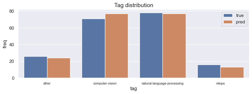
1 2 3 4 5 | |
100%|██████████| 191/191 [02:28<00:00,  1.29it/s]
{
  "precision": 0.9314722577069027,
  "recall": 0.9267015706806283,
  "f1": 0.9271956481845013
}
Few-shot learning
Now, we'll be adding a assistant_context with a few samples from our training data for each class. The intuition here is that we're giving the model a few examples (few-shot learning) of what each class looks like so that it can learn to generalize better.
1 2 3 4 5 6 7 8 | |
[{'title': 'Comparison between YOLO and RCNN on real world videos',
  'description': 'Bringing theory to experiment is cool. We can easily train models in colab and find the results in minutes.',
  'tag': 'computer-vision'},
 {'title': 'Show, Infer & Tell: Contextual Inference for Creative Captioning',
  'description': 'The beauty of the work lies in the way it architects the fundamental idea that humans look at the overall image and then individual pieces of it.\r\n',
  'tag': 'computer-vision'},
 {'title': 'Awesome Graph Classification',
  'description': 'A collection of important graph embedding, classification and representation learning papers with implementations.',
  'tag': 'other'},
 {'title': 'Awesome Monte Carlo Tree Search',
  'description': 'A curated list of Monte Carlo tree search papers with implementations. ',
  'tag': 'other'},
 {'title': 'Rethinking Batch Normalization in Transformers',
  'description': 'We found that NLP batch statistics exhibit large variance throughout training, which leads to poor BN performance.',
  'tag': 'natural-language-processing'},
 {'title': 'ELECTRA: Pre-training Text Encoders as Discriminators',
  'description': 'PyTorch implementation of the electra model from the paper: ELECTRA - Pre-training Text Encoders as Discriminators Rather Than Generators',
  'tag': 'natural-language-processing'},
 {'title': 'Pytest Board',
  'description': 'Continuous pytest runner with awesome visualization.',
  'tag': 'mlops'},
 {'title': 'Debugging Neural Networks with PyTorch and W&B',
  'description': 'A closer look at debugging common issues when training neural networks.',
  'tag': 'mlops'}]
1 2 3 | |
Here are some examples with the correct labels: [{'title': 'Comparison between YOLO and RCNN on real world videos', ... 'description': 'A closer look at debugging common issues when training neural networks.', 'tag': 'mlops'}]
Tip
We could increase the number of samples by increasing the context length. We could also retrieve better few-shot samples by extracting examples from the training data that are similar to the current sample (ex. similar unique vocabulary).
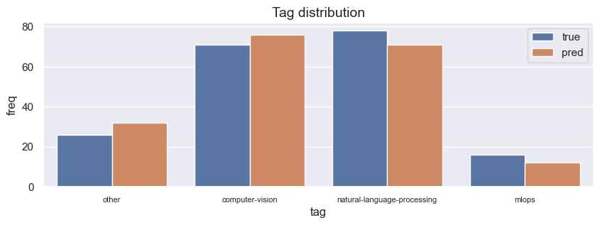
1 2 3 4 5 6 | |
100%|██████████| 191/191 [04:18<00:00,  1.35s/it]
{
  "precision": 0.8435247936255214,
  "recall": 0.8586387434554974,
  "f1": 0.8447984162323493
}
1 2 3 4 5 6 | |
100%|██████████| 191/191 [02:11<00:00,  1.46it/s]
{
  "precision": 0.9407759040163695,
  "recall": 0.9267015706806283,
  "f1": 0.9302632275594479
}
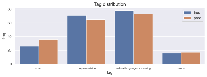
As we can see, few shot learning performs better than it's respective zero shot counter part. GPT 4 has had considerable improvements in reducing hallucinations but for our supervised task this comes at an expense of high precision but lower recall and f1 scores. When GPT 4 is not confident, it would rather predict other.
OSS LLMs
So far, we've only been using closed-source models from OpenAI. While these are currently the gold-standard, there are many open-source models that are rapidly catching up (Falcon 40B, Llama 2, etc.). Before we see how these models perform on our task, let's first consider a few reasons why we should care about open-source models.
- data ownership: you can serve your models and pass data to your models, without having to share it with a third-party API endpoint.
- fine-tune: with access to our model's weights, we can actually fine-tune them, as opposed to experimenting with fickle prompting strategies.
- optimization: we have full freedom to optimize our deployed models for inference (ex. quantization, pruning, etc.) to reduce costs.
1 | |
Results
Now let's compare all the results from our generative AI LLM benchmarks:
1 | |
{
  "zero_shot": {
    "gpt-3.5-turbo-0613": {
      "precision": 0.7919133278407181,
      "recall": 0.806282722513089,
      "f1": 0.7807530967691199
    },
    "gpt-4-0613": {
      "precision": 0.9314722577069027,
      "recall": 0.9267015706806283,
      "f1": 0.9271956481845013
    }
  },
  "few_shot": {
    "gpt-3.5-turbo-0613": {
      "precision": 0.8435247936255214,
      "recall": 0.8586387434554974,
      "f1": 0.8447984162323493
    },
    "gpt-4-0613": {
      "precision": 0.9407759040163695,
      "recall": 0.9267015706806283,
      "f1": 0.9302632275594479
    }
  }
}
And we can plot these on a bar plot to compare them visually.
1 2 3 4 5 6 | |
1 2 3 4 5 6 7 8 9 10 11 12 13 14 15 16 17 18 19 20 21 22 23 24 | |
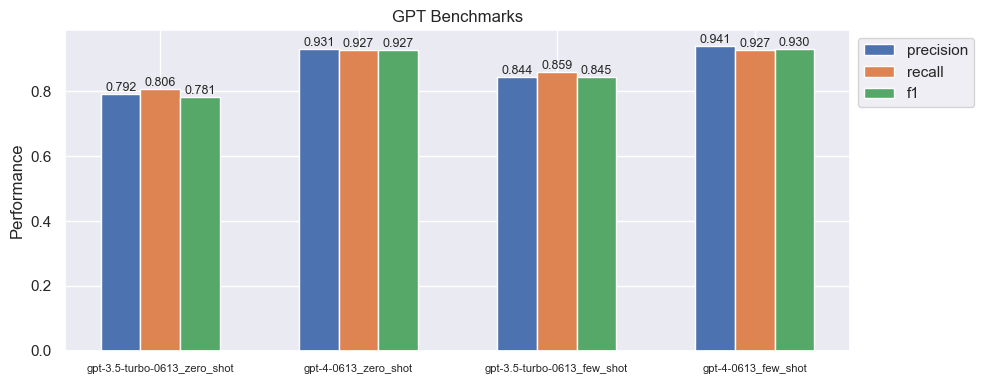
Our best model is GPT 4 with few shot learning at an f1 score of ~93%. We will see, in the rest of the course, how fine-tuning an LLM with a proper training dataset to change the actual weights of the last N layers (as opposed to the hard prompt tuning here) will yield similar/slightly better results to GPT 4 (at a fraction of the model size and inference costs).
However, the best system might actually be a combination of using these few-shot hard prompt LLMs alongside fine-tuned LLMs. For example, our fine-tuned LLMs in the course will perform well when the test data is similar to the training data (similar distributions of vocabulary, etc.) but may not perform well on out of distribution. Whereas, these hard prompted LLMs, by themselves or augmented with additional context (ex. arXiv plugins in our case), could be used when our primary fine-tuned model is not so confident.
Setup
We'll start by defining some setup utilities and configuring our model.
1 2 3 4 | |
We'll define a set_seeds function that will set the seeds for reproducibility across our libraries (np.random.seed, random.seed, torch.manual_seed and torch.cuda.manual_seed). We'll also set the behavior for some torch backends to ensure deterministic results when we run our workloads on GPUs.
1 2 3 4 5 6 7 8 9 | |
Next, we'll define a simple load_data function to ingest our data from source (CSV files) and load it as a Ray Dataset.
1 2 3 4 5 | |
Tip
When working with very large datasets, it's a good idea to limit the number of samples in our dataset so that we can execute our code quickly and iterate on bugs, etc. This is why we have a num_samples input argument in our load_data function (None = no limit, all samples).
We'll also define a custom preprocessor class that we'll to conveniently preprocess our dataset but also to save/load for later. When defining a preprocessor, we'll need to define a _fit method to learn how to fit to our dataset and a _transform_{pandas|numpy} method to preprocess the dataset using any components from the _fit method. We can either define a _transform_pandas method to apply our preprocessing to a Pandas DataFrame or a _transform_numpy method to apply our preprocessing to a NumPy array. We'll define the _transform_pandas method since our preprocessing function expects a batch of data as a Pandas DataFrame.
1 2 3 4 5 6 7 8 | |
Model
Now we're ready to start defining our model architecture. We'll start by loading a pretrained LLM and then defining the components needed for fine-tuning it on our dataset. Our pretrained LLM here is a transformer-based model that has been pretrained on a large corpus of scientific text called scibert.

If you're not familiar with transformer-based models like LLMs, be sure to check out the attention and Transformers lessons.
1 2 | |
We can load our pretrained model by using the from_pretrained` method.
1 2 3 | |
Once our model is loaded, we can tokenize an input text, convert it to torch tensors and pass it through our model to get a sequence and pooled representation of the text.
1 2 3 4 5 6 | |
(torch.Size([1, 10, 768]), torch.Size([1, 768]))
We're going to use this pretrained model to represent our input text features and add additional layers (linear classifier) on top of it for our specific classification task. In short, the pretrained LLM will process the tokenized text and return a sequence (one representation after each token) and pooled (combined) representation of the text. We'll use the pooled representation as input to our final fully-connection layer (fc1) to result in a vector of size num_classes (number of classes) that we can use to make predictions.
1 2 3 4 5 6 7 8 9 10 11 12 13 14 15 16 17 18 19 20 21 22 23 24 25 26 27 | |
Let's initialize our model and inspect its layers:
1 2 3 | |
(llm): BertModel(
(embeddings): BertEmbeddings(
    (word_embeddings): Embedding(31090, 768, padding_idx=0)
    (position_embeddings): Embedding(512, 768)
    (token_type_embeddings): Embedding(2, 768)
    (LayerNorm): LayerNorm((768,), eps=1e-12, elementwise_affine=True)
    (dropout): Dropout(p=0.1, inplace=False)
)
(encoder): BertEncoder(
    (layer): ModuleList(
    (0-11): 12 x BertLayer(
        (attention): BertAttention(
        (self): BertSelfAttention(
            (query): Linear(in_features=768, out_features=768, bias=True)
            (key): Linear(in_features=768, out_features=768, bias=True)
            (value): Linear(in_features=768, out_features=768, bias=True)
            (dropout): Dropout(p=0.1, inplace=False)
        )
        (output): BertSelfOutput(
            (dense): Linear(in_features=768, out_features=768, bias=True)
            (LayerNorm): LayerNorm((768,), eps=1e-12, elementwise_affine=True)
            (dropout): Dropout(p=0.1, inplace=False)
        )
        )
        (intermediate): BertIntermediate(
        (dense): Linear(in_features=768, out_features=3072, bias=True)
        (intermediate_act_fn): GELUActivation()
        )
        (output): BertOutput(
        (dense): Linear(in_features=3072, out_features=768, bias=True)
        (LayerNorm): LayerNorm((768,), eps=1e-12, elementwise_affine=True)
        (dropout): Dropout(p=0.1, inplace=False)
        )
    )
    )
)
(pooler): BertPooler(
    (dense): Linear(in_features=768, out_features=768, bias=True)
    (activation): Tanh()
)
)
(dropout): Dropout(p=0.5, inplace=False)
(fc1): Linear(in_features=768, out_features=4, bias=True)
Batching
We can iterate through our dataset in batches however we may have batches of different sizes. Recall that our tokenizer padded the inputs to the longest item in the batch (padding="longest"). However, our batches for training will be smaller than our large data processing batches and so our batches here may have inputs with different lengths. To address this, we're going to define a custom collate_fn to repad the items in our training batches.
1 | |
Our pad_array function will take an array of arrays and pad the inner arrays to the longest length.
1 2 3 4 5 6 | |
And our collate_fn will take a batch of data to pad them and convert them to the appropriate PyTorch tensor types.
1 2 3 4 5 6 7 8 | |
Let's test our collate_fn on a sample batch from our dataset.
1 2 3 | |
{'ids': tensor([[  102,  5800, 14982,  ...,     0,     0,     0],
         [  102,  7746,  2824,  ...,     0,     0,     0],
         [  102,   502,  1371,  ...,     0,     0,     0],
         ...,
         [  102, 10431,   160,  ...,     0,     0,     0],
         [  102,   124,   132,  ...,     0,     0,     0],
         [  102, 12459, 28196,  ...,     0,     0,     0]], dtype=torch.int32),
 'masks': tensor([[1, 1, 1,  ..., 0, 0, 0],
         [1, 1, 1,  ..., 0, 0, 0],
         [1, 1, 1,  ..., 0, 0, 0],
         ...,
         [1, 1, 1,  ..., 0, 0, 0],
         [1, 1, 1,  ..., 0, 0, 0],
         [1, 1, 1,  ..., 0, 0, 0]], dtype=torch.int32),
 'targets': tensor([2, 0, 3, 2, 0, 3, 2, 0, 2, 0, 2, 2, 0, 3, 2, 0, 2, 3, 0, 2, 2, 0, 2, 2,
         0, 1, 1, 0, 2, 0, 3, 2, 0, 3, 2, 0, 2, 0, 2, 2, 0, 2, 0, 3, 2, 0, 3, 2,
         0, 2, 0, 2, 2, 0, 3, 2, 0, 2, 3, 0, 2, 2, 0, 2, 2, 0, 1, 1, 0, 3, 0, 0,
         0, 3, 0, 1, 1, 0, 3, 2, 0, 2, 3, 0, 2, 2, 0, 2, 2, 0, 1, 1, 0, 3, 2, 0,
         2, 3, 0, 2, 2, 0, 2, 2, 0, 1, 1, 0, 2, 0, 2, 2, 0, 2, 2, 0, 2, 0, 1, 1,
         0, 0, 0, 1, 0, 0, 1, 0])}
Utilities
Next, we'll implement set the necessary utility functions for distributed training.

1 2 3 4 5 | |
We'll start by defining what one step (or iteration) of training looks like. This will be a function that takes in a batch of data, a model, a loss function, and an optimizer. It will then perform a forward pass, compute the loss, and perform a backward pass to update the model's weights. And finally, it will return the loss.
1 2 3 4 5 6 7 8 9 10 11 12 13 14 | |
Note: We're using the
ray.data.iter_torch_batchesmethod instead oftorch.utils.data.DataLoaderto create a generator that will yield batches of data. In fact, this is the only line that's different from a typical PyTorch training loop and the actual training workflow remains untouched. Ray supports many other ways to load/consume data for different frameworks as well.
The validation step is quite similar to the training step but we don't need to perform a backward pass or update the model's weights.
1 2 3 4 5 6 7 8 9 10 11 12 13 14 15 | |
Next, we'll define the train_loop_per_worker which defines the overall training loop for each worker. It's important that we include operations like loading the datasets, models, etc. so that each worker will have its own copy of these objects. Ray takes care of combining all the workers' results at the end of each iteration, so from the user's perspective, it's the exact same as training on a single machine!
The only additional lines of code we need to add compared to a typical PyTorch training loop are the following:
session.get_dataset_shard("train")andsession.get_dataset_shard("val")to load the data splits (session.get_dataset_shard).model = train.torch.prepare_model(model)to prepare the torch model for distributed execution (train.torch.prepare_model).batch_size_per_worker = batch_size // session.get_world_size()to adjust the batch size for each worker (session.get_world_size).session.report(metrics, checkpoint=checkpoint)to report metrics and save our model checkpoint (session.report).
All the other lines of code are the same as a typical PyTorch training loop!
1 2 3 4 5 6 7 8 9 10 11 12 13 14 15 16 17 18 19 20 21 22 23 24 25 26 27 28 29 30 31 32 33 34 35 36 37 38 | |
Class imbalance
Our dataset doesn't suffer from horrible class imbalance, but if it did, we could easily account for it through our loss function. There are also other strategies such as over-sampling less frequent classes and under-sampling popular classes.
1 2 3 4 5 6 7 8 9 10 11 | |
Configurations
Next, we'll define some configurations that will be used to train our model.
1 2 3 4 5 6 7 8 9 10 | |
Next we'll define our scaling configuration (ScalingConfig) that will specify how we want to scale our training workload. We specify the number of workers (num_workers), whether to use GPU or not (use_gpu), the resources per worker (resources_per_worker) and how much CPU each worker is allowed to use (_max_cpu_fraction_per_node).
1 2 3 4 5 6 7 | |
_max_cpu_fraction_per_node=0.8indicates that 20% of CPU is reserved for non-training workloads that our workers will do such as data preprocessing (which we do prior to training anyway).
Next, we'll define our CheckpointConfig which will specify how we want to checkpoint our model. Here we will just save one checkpoint (num_to_keep) based on the checkpoint with the min val_loss. We'll also configure a RunConfig which will specify the name of our run and where we want to save our checkpoints.
1 2 3 | |
We'll be naming our experiment llm and saving our results to ~/ray_results, so a sample directory structure for our trained models would look like this:
/home/ray/ray_results/llm
├── TorchTrainer_fd40a_00000_0_2023-07-20_18-14-50/
├── basic-variant-state-2023-07-20_18-14-50.json
├── experiment_state-2023-07-20_18-14-50.json
├── trainer.pkl
└── tuner.pkl
The TorchTrainer_ objects are the individuals runs in this experiment and each one will have the following contents:
/home/ray/ray_results/TorchTrainer_fd40a_00000_0_2023-07-20_18-14-50/
├── checkpoint_000009/  # we only save one checkpoint (the best)
├── events.out.tfevents.1689902160.ip-10-0-49-200
├── params.json
├── params.pkl
├── progress.csv
└── result.json
There are several other configs that we could set with Ray (ex. failure handling) so be sure to check them out here.
Stopping criteria
While we'll just let our experiments run for a certain number of epochs and stop automatically, our RunConfig accepts an optional stopping criteria (stop) which determines the conditions our training should stop for. It's entirely customizable and common examples include a certain metric value, elapsed time or even a custom class.
Training
Now we're finally ready to train our model using all the components we've setup above.
1 2 3 | |
1 2 3 4 5 6 | |
Calling materialize here is important because it will cache the preprocessed data in memory. This will allow us to train our model without having to reprocess the data each time.
Because we've preprocessed the data prior to training, we can use the fit=False and transform=False flags in our dataset config. This will allow us to skip the preprocessing step during training.
1 2 3 4 5 | |
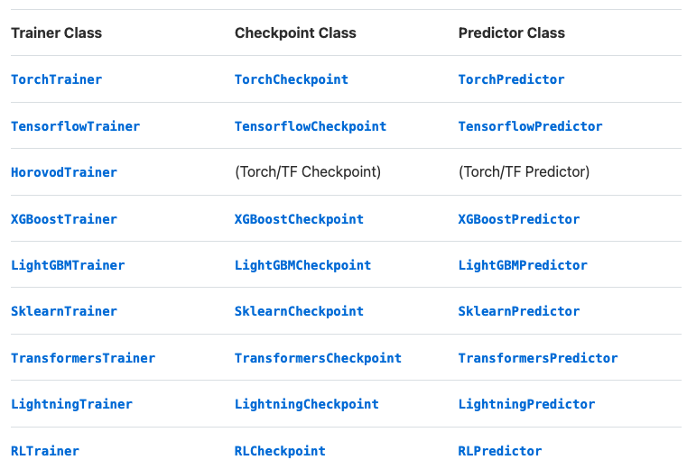
We'll pass all of our functions and configs to the TorchTrainer class to start training. Ray supports a wide variety of framework Trainers so if you're using other frameworks, you can use the corresponding Trainer class instead.
1 2 3 4 5 6 7 8 9 10 | |
Now let's fit our model to the data.
1 2 | |
1 | |
1 | |
[(TorchCheckpoint(local_path=/home/ray/ray_results/llm/TorchTrainer_8c960_00000_0_2023-07-10_16-14-41/checkpoint_000009),
  {'epoch': 9,
   'lr': 0.0001,
   'train_loss': 0.0005496611799268673,
   'val_loss': 0.0011818759376183152,
   'timestamp': 1689030958,
   'time_this_iter_s': 6.604866981506348,
   'should_checkpoint': True,
   'done': True,
   'training_iteration': 10,
   'trial_id': '8c960_00000',
   'date': '2023-07-10_16-16-01',
   'time_total_s': 76.30888652801514,
   'pid': 68577,
   'hostname': 'ip-10-0-18-44',
   'node_ip': '10.0.18.44',
   'config': {'train_loop_config': {'dropout_p': 0.5,
     'lr': 0.0001,
     'lr_factor': 0.8,
     'lr_patience': 3,
     'num_epochs': 10,
     'batch_size': 256,
     'num_classes': 4}},
   'time_since_restore': 76.30888652801514,
   'iterations_since_restore': 10,
   'experiment_tag': '0'})]
Observability
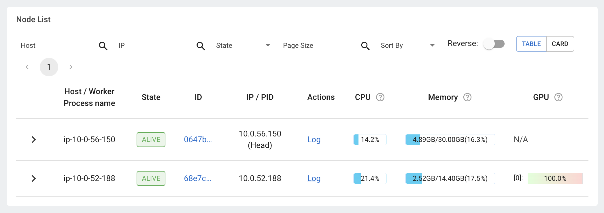
While our model is training, we can inspect our Ray dashboard to observe how our compute resources are being utilized.
💻 Local
We can inspect our Ray dashboard by opening http://127.0.0.1:8265 on a browser window. Click on Cluster on the top menu bar and then we will be able to see a list of our nodes (head and worker) and their utilizations.
🚀 Anyscale
On Anyscale Workspaces, we can head over to the top right menu and click on 🛠️ Tools → Ray Dashboard and this will open our dashboard on a new tab. Click on Cluster on the top menu bar and then we will be able to see a list of our nodes (head and worker) and their utilizations.
Learn about all the other observability features on the Ray Dashboard through this video.
Evaluation
Now that we've trained our model, we can evaluate it on a separate holdout test set. We'll cover the topic of evaluation much more extensively in our evaluation lesson but for now we'll calculate some quick overall metrics.
1 2 | |
We'll define a function that can take in a dataset and a predictor and return the performance metrics.
- Load the predictor and preprocessor from the best checkpoint:
1
2
3
4
# Predictor best_checkpoint = results.best_checkpoints[0][0] predictor = TorchPredictor.from_checkpoint(best_checkpoint) preprocessor = predictor.get_preprocessor() - Load and preprocess the test dataset that we want to evaluate on:
1
2
3
4
5
# Test (holdout) dataset
HOLDOUT_LOC = "https://raw.githubusercontent.com/GokuMohandas/Made-With-ML/main/datasets/holdout.csv"
test_ds = ray.data.read_csv(HOLDOUT_LOC)
preprocessed_ds = preprocessor.transform(test_ds)
preprocessed_ds.take(1)
[{'ids': array([  102,  4905,  2069,  2470,  2848,  4905, 30132, 22081,   691,
          4324,  7491,  5896,   341,  6136,   934, 30137,   103,     0,
             0,     0,     0]),
  'masks': array([1, 1, 1, 1, 1, 1, 1, 1, 1, 1, 1, 1, 1, 1, 1, 1, 1, 0, 0, 0, 0]),
  'targets': 3}]
- Retrieve the true label indices from the
targetscolumn by using ray.data.Dataset.select_column:1 2 3 4
# y_true values = preprocessed_ds.select_columns(cols=["targets"]).take_all() y_true = np.stack([item["targets"] for item in values]) print (y_true)
[3 3 3 0 2 0 0 0 0 2 0 0 2 3 0 0 2 2 3 2 3 0 3 2 0 2 2 1 1 2 2 2 2 2 2 0 0 0 0 0 1 1 2 0 0 3 1 2 0 2 2 3 3 0 2 3 2 3 3 3 3 0 0 0 0 2 2 0 2 1 0 2 3 0 0 2 2 2 2 2 0 0 2 0 1 0 0 0 0 3 0 0 2 0 2 2 3 2 0 2 0 2 0 3 0 0 0 0 0 2 0 0 2 2 2 2 3 0 2 0 2 0 2 3 3 3 2 0 2 2 2 2 0 2 2 2 0 1 2 2 2 2 2 1 2 0 3 0 2 2 1 1 2 0 0 0 0 0 0 2 2 2 0 2 1 1 2 0 0 1 2 3 2 2 2 0 0 2 0 2 0 3 0 2 2 0 1 2 1 2 2]
- Get our predicted label indices by using the
predictor. Note that thepredictorwill automatically take care of the preprocessing for us.1 2 3 4
# y_pred z = predictor.predict(data=test_ds.to_pandas())["predictions"] y_pred = np.stack(z).argmax(1) print (y_pred)
[3 3 3 0 2 0 0 0 0 2 0 0 2 3 0 0 0 2 3 2 3 0 3 2 0 0 2 1 1 2 2 2 2 2 2 0 0 0 0 0 1 2 2 0 2 3 1 2 0 2 2 3 3 0 2 1 2 3 3 3 3 2 0 0 0 2 2 0 2 1 0 2 3 1 0 2 2 2 2 2 0 0 2 1 1 0 0 0 0 3 0 0 2 0 2 2 3 2 0 2 0 2 2 0 2 0 0 3 0 2 0 0 1 2 2 2 3 0 2 0 2 0 2 3 3 3 2 0 2 2 2 2 0 2 2 2 0 1 2 2 2 2 2 1 2 0 3 0 2 2 2 1 2 0 2 0 0 0 0 2 2 2 0 2 1 2 2 0 0 1 2 3 2 2 2 0 0 2 0 2 1 3 0 2 2 0 1 2 1 2 2]
- Compute our metrics using the true and predicted labels indices.
1 2 3
# Evaluate metrics = precision_recall_fscore_support(y_true, y_pred, average="weighted") {"precision": metrics[0], "recall": metrics[1], "f1": metrics[2]}
{'precision': 0.9147673308349523,
'recall': 0.9109947643979057,
'f1': 0.9115810676649443}
We're going to encapsulate all of these steps into one function so that we can call on it as we train more models soon.
1 2 3 4 5 6 7 8 9 10 11 12 13 14 15 | |
Inference
Now let's load our trained model for inference on new data. We'll create a few utility functions to format the probabilities into a dictionary for each class and to return predictions for each item in a dataframe.
1 | |
1 2 3 4 5 | |
1 2 3 4 5 6 7 8 9 | |
We'll load our predictor from the best checkpoint and load it's preprocessor.
1 2 3 | |
And now we're ready to apply our model to new data. We'll create a sample dataframe with a title and description and then use our predict_with_proba function to get the predictions. Note that we use a placeholder value for tag since our input dataframe will automatically be preprocessed (and it expects a value in the tag column).
1 2 3 4 5 | |
[{'prediction': 'natural-language-processing',
'probabilities': {'computer-vision': 0.0007296873,
'mlops': 0.0008382588,
'natural-language-processing': 0.997829,
'other': 0.00060295867}}]
Optimization
Distributed training strategies are great for when our data or models are too large for training but there are additional strategies to make the models itself smaller for serving. The following model compression techniques are commonly used to reduce the size of the model:
- Pruning: remove weights (unstructured) or entire channels (structured) to reduce the size of the network. The objective is to preserve the model’s performance while increasing its sparsity.
- Quantization: reduce the memory footprint of the weights by reducing their precision (ex. 32 bit to 8 bit). We may loose some precision but it shouldn’t affect performance too much.
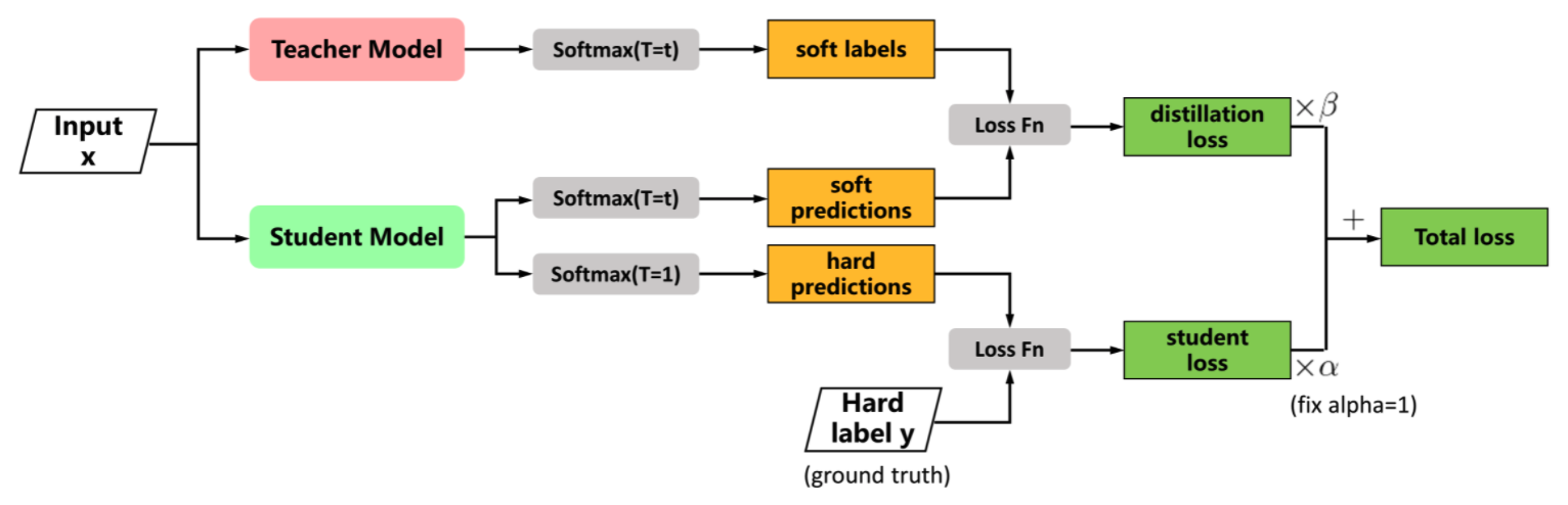
- Distillation: training smaller networks to “mimic” larger networks by having it reproduce the larger network’s layers’ outputs.
Upcoming live cohorts
Sign up for our upcoming live cohort, where we'll provide live lessons + QA, compute (GPUs) and community to learn everything in one day.
To cite this content, please use:
1 2 3 4 5 6 | |