Linear Regression

View all lessons

---

Implement linear regression from scratch using NumPy and then using PyTorch.

Goku Mohandas

· · ·

Repository · Notebook

×

Subscribe to our newsletter

📬  Receive new lessons straight to your inbox (once a month) and join 40K+ developers in learning how to responsibly deliver value with ML.

Subscribe

---

Overview

Our goal is to learn a linear model \(\hat{y}\) that models \(y\) given \(X\) using weights \(W\) and bias \(b\):

\[ \hat{y} = XW + b \]

Variable	Description
\(N\)	total numbers of samples
\(\hat{y}\)	predictions \(\in \mathbb{R}^{NX1}\)
\(X\)	inputs \(\in \mathbb{R}^{NXD}\)
\(W\)	weights \(\in \mathbb{R}^{DX1}\)
\(b\)	bias \(\in \mathbb{R}^{1}\)

• Objective:
  • Use inputs \(X\) to predict the output \(\hat{y}\) using a linear model. The model will be a line of best fit that minimizes the distance between the predicted (model's output) and target (ground truth) values. Training data \((X, y)\) is used to train the model and learn the weights \(W\) using gradient descent.
• Advantages:
  • Computationally simple.
  • Highly interpretable.
  • Can account for continuous and categorical features.
• Disadvantages:
  • The model will perform well only when the data is linearly separable (for classification).
• Miscellaneous:
  • You can also use linear regression for binary classification tasks where if the predicted continuous value is above a threshold, it belongs to a certain class. But we will cover better techniques for classification in future lessons and will focus on linear regression for continuous regression tasks only.

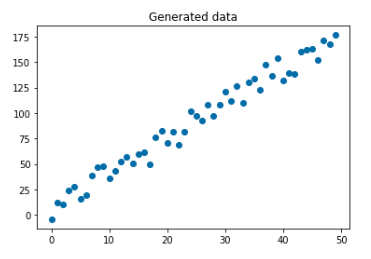
Generate data

We're going to generate some simple dummy data to apply linear regression on. It's going to create roughly linear data (y = 3.5X + noise); the random noise is added to create realistic data that doesn't perfectly align in a line. Our goal is to have the model converge to a similar linear equation (there will be slight variance since we added some noise).

import numpy as np
import pandas as pd
import matplotlib.pyplot as plt

SEED = 1234
NUM_SAMPLES = 50

# Set seed for reproducibility
np.random.seed(SEED)

# Generate synthetic data
def generate_data(num_samples):
    """Generate dummy data for linear regression."""
    X = np.array(range(num_samples))
    random_noise = np.random.uniform(-10, 20, size=num_samples)
    y = 3.5*X + random_noise # add some noise
    return X, y

# Generate random (linear) data
X, y = generate_data(num_samples=NUM_SAMPLES)
data = np.vstack([X, y]).T
print (data[:5])

[[ 0.         -4.25441649]
 [ 1.         12.16326313]
 [ 2.         10.13183217]
 [ 3.         24.06075751]
 [ 4.         27.39927424]]

# Load into a Pandas DataFrame
df = pd.DataFrame(data, columns=["X", "y"])
X = df[["X"]].values
y = df[["y"]].values
df.head()

	X	y
0	0.0	-4.254416
1	1.0	12.163263
2	2.0	10.131832
3	3.0	24.060758
4	4.0	27.399274

# Scatter plot
plt.title("Generated data")
plt.scatter(x=df["X"], y=df["y"])
plt.show()

NumPy

Now that we have our data prepared, we'll first implement linear regression using just NumPy. This will let us really understand the underlying operations.

Split data

Since our task is a regression task, we will randomly split our dataset into three sets: train, validation and test data splits.

• train: used to train our model.
• val : used to validate our model's performance during training.
• test: used to do an evaluation of our fully trained model.

Be sure to check out our entire lesson focused on properly splitting data in our MLOps course.

TRAIN_SIZE = 0.7
VAL_SIZE = 0.15
TEST_SIZE = 0.15

# Shuffle data
indices = list(range(NUM_SAMPLES))
np.random.shuffle(indices)
X = X[indices]
y = y[indices]

Warning

Be careful not to shuffle \(X\) and \(y\) separately because then the inputs won't correspond to the outputs!

# Split indices
train_start = 0
train_end = int(0.7*NUM_SAMPLES)
val_start = train_end
val_end = int((TRAIN_SIZE+VAL_SIZE)*NUM_SAMPLES)
test_start = val_end

# Split data
X_train = X[train_start:train_end]
y_train = y[train_start:train_end]
X_val = X[val_start:val_end]
y_val = y[val_start:val_end]
X_test = X[test_start:]
y_test = y[test_start:]
print (f"X_train: {X_train.shape}, y_train: {y_train.shape}")
print (f"X_val: {X_val.shape}, y_test: {y_val.shape}")
print (f"X_test: {X_test.shape}, y_test: {y_test.shape}")

X_train: (35, 1), y_train: (35, 1)
X_val: (7, 1), y_test: (7, 1)
X_test: (8, 1), y_test: (8, 1)

Standardize data

We need to standardize our data (zero mean and unit variance) so a specific feature's magnitude doesn't affect how the model learns its weights.

\[ z = \frac{x_i - \mu}{\sigma} \]

Variable	Description
\(z\)	standardized value
\(x_i\)	inputs
\(\mu\)	mean
\(\sigma\)	standard deviation

def standardize_data(data, mean, std):
    return (data - mean)/std

# Determine means and stds
X_mean = np.mean(X_train)
X_std = np.std(X_train)
y_mean = np.mean(y_train)
y_std = np.std(y_train)

We need to treat the validation and test sets as if they were hidden datasets. So we only use the train set to determine the mean and std to avoid biasing our training process.

# Standardize
X_train = standardize_data(X_train, X_mean, X_std)
y_train = standardize_data(y_train, y_mean, y_std)
X_val = standardize_data(X_val, X_mean, X_std)
y_val = standardize_data(y_val, y_mean, y_std)
X_test = standardize_data(X_test, X_mean, X_std)
y_test = standardize_data(y_test, y_mean, y_std)

# Check (means should be ~0 and std should be ~1)
# Check (means should be ~0 and std should be ~1)
print (f"mean: {np.mean(X_test, axis=0)[0]:.1f}, std: {np.std(X_test, axis=0)[0]:.1f}")
print (f"mean: {np.mean(y_test, axis=0)[0]:.1f}, std: {np.std(y_test, axis=0)[0]:.1f}")

mean: -0.4, std: 0.9
mean: -0.3, std: 1.0

Weights

Our goal is to learn a linear model \(\hat{y}\) that models \(y\) given \(X\) using weights \(W\) and bias \(b\) → \(\hat{y} = XW + b\)

Step 1: Randomly initialize the model's weights \(W\).

INPUT_DIM = X_train.shape[1] # X is 1-dimensional
OUTPUT_DIM = y_train.shape[1] # y is 1-dimensional

# Initialize random weights
W = 0.01 * np.random.randn(INPUT_DIM, OUTPUT_DIM)
b = np.zeros((1, 1))
print (f"W: {W.shape}")
print (f"b: {b.shape}")

W: (1, 1)
b: (1, 1)

Model

Step 2: Feed inputs \(X\) into the model to receive the predictions \(\hat{y}\)

# Forward pass [NX1] · [1X1] = [NX1]
y_pred = np.dot(X_train, W) + b
print (f"y_pred: {y_pred.shape}")

y_pred: (35, 1)

Loss

Step 3: Compare the predictions \(\hat{y}\) with the actual target values \(y\) using the objective (cost) function to determine the loss \(J\). A common objective function for linear regression is mean squared error (MSE). This function calculates the difference between the predicted and target values and squares it.

\[ J(\theta) = \frac{1}{N} \sum_i (y_i - \hat{y}_i)^2 = \frac{1}{N}\sum_i (y_i - X_iW)^2 \]

bias term (\(b\)) excluded to avoid crowding the notations

# Loss
N = len(y_train)
loss = (1/N) * np.sum((y_train - y_pred)**2)
print (f"loss: {loss:.2f}")

loss: 0.99

Gradients

Step 4: Calculate the gradient of loss \(J(\theta)\) w.r.t to the model weights.

\[ → \frac{\partial{J}}{\partial{W}} = -\frac{2}{N} \sum_i (y_i - X_iW) X_i = -\frac{2}{N} \sum_i (y_i - \hat{y}_i) X_i \]

\[ → \frac{\partial{J}}{\partial{b}} = -\frac{2}{N} \sum_i (y_i - X_iW)1 = -\frac{2}{N} \sum_i (y_i - \hat{y}_i)1 \]

# Backpropagation
dW = -(2/N) * np.sum((y_train - y_pred) * X_train)
db = -(2/N) * np.sum((y_train - y_pred) * 1)

The gradient is the derivative, or the rate of change of a function. It's a vector that points in the direction of greatest increase of a function. For example the gradient of our loss function (\(J\)) with respect to our weights (\(W\)) will tell us how to change \(W\) so we can maximize \(J\). However, we want to minimize our loss so we subtract the gradient from \(W\).

Update weights

Step 5: Update the weights \(W\) using a small learning rate \(\alpha\).

\[ W = W - \alpha\frac{\partial{J}}{\partial{W}} \]

\[ b = b - \alpha\frac{\partial{J}}{\partial{b}} \]

LEARNING_RATE = 1e-1

# Update weights
W += -LEARNING_RATE * dW
b += -LEARNING_RATE * db

The learning rate \(\alpha\) is a way to control how much we update the weights by. If we choose a small learning rate, it may take a long time for our model to train. However, if we choose a large learning rate, we may overshoot and our training will never converge. The specific learning rate depends on our data and the type of models we use but it's typically good to explore in the range of \([1e^{-8}, 1e^{-1}]\). We'll explore learning rate update strategies in later lessons.

Training

Step 6: Repeat steps 2 - 5 to minimize the loss and train the model.

NUM_EPOCHS = 100

# Initialize random weights
W = 0.01 * np.random.randn(INPUT_DIM, OUTPUT_DIM)
b = np.zeros((1, ))

# Training loop
for epoch_num in range(NUM_EPOCHS):

    # Forward pass [NX1] · [1X1] = [NX1]
    y_pred = np.dot(X_train, W) + b

    # Loss
    loss = (1/len(y_train)) * np.sum((y_train - y_pred)**2)

    # Show progress
    if epoch_num%10 == 0:
        print (f"Epoch: {epoch_num}, loss: {loss:.3f}")

    # Backpropagation
    dW = -(2/N) * np.sum((y_train - y_pred) * X_train)
    db = -(2/N) * np.sum((y_train - y_pred) * 1)

    # Update weights
    W += -LEARNING_RATE * dW
    b += -LEARNING_RATE * db

Epoch: 0, loss: 0.990
Epoch: 10, loss: 0.039
Epoch: 20, loss: 0.028
Epoch: 30, loss: 0.028
Epoch: 40, loss: 0.028
Epoch: 50, loss: 0.028
Epoch: 60, loss: 0.028
Epoch: 70, loss: 0.028
Epoch: 80, loss: 0.028
Epoch: 90, loss: 0.028

To keep the code simple, we're not calculating and displaying the validation loss after each epoch here. But in later lessons, the performance on the validation set will be crucial in influencing the learning process (learning rate, when to stop training, etc.).

Evaluation

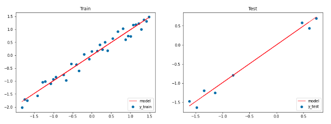
Now we're ready to see how well our trained model will perform on our test (hold-out) data split. This will be our best measure on how well the model would perform on the real world, given that our dataset's distribution is close to unseen data.

# Predictions
pred_train = W*X_train + b
pred_test = W*X_test + b

# Train and test MSE
train_mse = np.mean((y_train - pred_train) ** 2)
test_mse = np.mean((y_test - pred_test) ** 2)
print (f"train_MSE: {train_mse:.2f}, test_MSE: {test_mse:.2f}")

train_MSE: 0.03, test_MSE: 0.01

# Figure size
plt.figure(figsize=(15,5))

# Plot train data
plt.subplot(1, 2, 1)
plt.title("Train")
plt.scatter(X_train, y_train, label="y_train")
plt.plot(X_train, pred_train, color="red", linewidth=1, linestyle="-", label="model")
plt.legend(loc="lower right")

# Plot test data
plt.subplot(1, 2, 2)
plt.title("Test")
plt.scatter(X_test, y_test, label='y_test')
plt.plot(X_test, pred_test, color="red", linewidth=1, linestyle="-", label="model")
plt.legend(loc="lower right")

# Show plots
plt.show()

Interpretability

Since we standardized our inputs and outputs, our weights were fit to those standardized values. So we need to unstandardize our weights so we can compare it to our true weight (3.5).

Note that both \(X\) and \(y\) were standardized.

\[ \hat{y}_{scaled} = b_{scaled} + \sum_{j=1}^{k}{W_{scaled}}_j{x_{scaled}}_j \]

Variable	Description
\(y_{scaled}\)	\(\frac{\hat{y} - \bar{y}}{\sigma_y}\)
\(x_{scaled}\)	\(\frac{x_j - \bar{x}_j}{\sigma_j}\)

\[ \frac{\hat{y} - \bar{y}}{\sigma_y} = b_{scaled} + \sum_{j=1}^{k}{W_{scaled}}_j\frac{x_j - \bar{x}_j}{\sigma_j} \]

\[ \hat{y}_{scaled} = \frac{\hat{y}_{unscaled} - \bar{y}}{\sigma_y} = {b_{scaled}} + \sum_{j=1}^{k} {W_{scaled}}_j (\frac{x_j - \bar{x}_j}{\sigma_j}) \]

\[ \hat{y}_{unscaled} = b_{scaled}\sigma_y + \bar{y} - \sum_{j=1}^{k} {W_{scaled}}_j(\frac{\sigma_y}{\sigma_j})\bar{x}_j + \sum_{j=1}^{k}{W_{scaled}}_j(\frac{\sigma_y}{\sigma_j})x_j \]

In the expression above, we can see the expression:

\[ \hat{y}_{unscaled} = b_{unscaled} + W_{unscaled}x \]

Variable	Description
\(W_{unscaled}\)	\({W}_j(\frac{\sigma_y}{\sigma_j})\)
\(b_{unscaled}\)	\(b_{scaled}\sigma_y + \bar{y} - \sum_{j=1}^{k} {W}_j(\frac{\sigma_y}{\sigma_j})\bar{x}_j\)

By substituting \(W_{unscaled}\) in \(b_{unscaled}\), it now becomes:

\[ b_{unscaled} = b_{scaled}\sigma_y + \bar{y} - \sum_{j=1}^{k} W_{unscaled}\bar{x}_j \]

# Unscaled weights
W_unscaled = W * (y_std/X_std)
b_unscaled = b * y_std + y_mean - np.sum(W_unscaled*X_mean)
print ("[actual] y = 3.5X + noise")
print (f"[model] y_hat = {W_unscaled[0][0]:.1f}X + {b_unscaled[0]:.1f}")

[actual] y = 3.5X + noise
[model] y_hat = 3.4X + 7.8

PyTorch

Now that we've implemented linear regression with Numpy, let's do the same with PyTorch.

import torch

# Set seed for reproducibility
torch.manual_seed(SEED)

Split data

This time, instead of splitting data using indices, let's use scikit-learn's built in train_test_split function.

from sklearn.model_selection import train_test_split

TRAIN_SIZE = 0.7
VAL_SIZE = 0.15
TEST_SIZE = 0.15

# Split (train)
X_train, X_, y_train, y_ = train_test_split(X, y, train_size=TRAIN_SIZE)

print (f"train: {len(X_train)} ({(len(X_train) / len(X)):.2f})\n"
       f"remaining: {len(X_)} ({(len(X_) / len(X)):.2f})")

train: 35 (0.70)
remaining: 15 (0.30)

# Split (test)
X_val, X_test, y_val, y_test = train_test_split(
    X_, y_, train_size=0.5)

print(f"train: {len(X_train)} ({len(X_train)/len(X):.2f})\n"
      f"val: {len(X_val)} ({len(X_val)/len(X):.2f})\n"
      f"test: {len(X_test)} ({len(X_test)/len(X):.2f})")

train: 35 (0.70)
val: 7 (0.14)
test: 8 (0.16)

Standardize data

This time we'll use scikit-learn's StandardScaler to standardize our data.

from sklearn.preprocessing import StandardScaler

# Standardize the data (mean=0, std=1) using training data
X_scaler = StandardScaler().fit(X_train)
y_scaler = StandardScaler().fit(y_train)

# Apply scaler on training and test data
X_train = X_scaler.transform(X_train)
y_train = y_scaler.transform(y_train).ravel().reshape(-1, 1)
X_val = X_scaler.transform(X_val)
y_val = y_scaler.transform(y_val).ravel().reshape(-1, 1)
X_test = X_scaler.transform(X_test)
y_test = y_scaler.transform(y_test).ravel().reshape(-1, 1)

# Check (means should be ~0 and std should be ~1)
print (f"mean: {np.mean(X_test, axis=0)[0]:.1f}, std: {np.std(X_test, axis=0)[0]:.1f}")
print (f"mean: {np.mean(y_test, axis=0)[0]:.1f}, std: {np.std(y_test, axis=0)[0]:.1f}")

mean: -0.3, std: 0.7
mean: -0.3, std: 0.6

Weights

We will be using PyTorch's Linear layers in our MLP implementation. These layers will act as out weights (and biases).

\[ z = XW \]

from torch import nn

# Inputs
N = 3 # num samples
x = torch.randn(N, INPUT_DIM)
print (x.shape)
print (x.numpy())

torch.Size([3, 1])
[[ 0.04613046]
 [ 0.40240282]
 [-1.0115291 ]]

# Weights
m = nn.Linear(INPUT_DIM, OUTPUT_DIM)
print (m)
print (f"weights ({m.weight.shape}): {m.weight[0][0]}")
print (f"bias ({m.bias.shape}): {m.bias[0]}")

Linear(in_features=1, out_features=1, bias=True)
weights (torch.Size([1, 1])): 0.35
bias (torch.Size([1])): -0.34

# Forward pass
z = m(x)
print (z.shape)
print (z.detach().numpy())

torch.Size([3, 1])
[[-0.32104054]
 [-0.19719592]
 [-0.68869597]]

Model

\[ \hat{y} = XW + b \]

class LinearRegression(nn.Module):
    def __init__(self, input_dim, output_dim):
        super(LinearRegression, self).__init__()
        self.fc1 = nn.Linear(input_dim, output_dim)

    def forward(self, x_in):
        y_pred = self.fc1(x_in)
        return y_pred

# Initialize model
model = LinearRegression(input_dim=INPUT_DIM, output_dim=OUTPUT_DIM)
print (model.named_parameters)

Model:
<bound method Module.named_parameters of LinearRegression(
  (fc1): Linear(in_features=1, out_features=1, bias=True)
)>

Loss

This time we're using PyTorch's loss functions, specifically MSELoss.

loss_fn = nn.MSELoss()
y_pred = torch.Tensor([0., 0., 1., 1.])
y_true =  torch.Tensor([1., 1., 1., 0.])
loss = loss_fn(y_pred, y_true)
print("Loss: ", loss.numpy())

Loss:  0.75

Optimizer

When we implemented linear regression with just NumPy, we used batch gradient descent to update our weights (used entire training set). But there are actually many different gradient descent optimization algorithms to choose from and it depends on the situation. However, the ADAM optimizer has become a standard algorithm for most cases.

from torch.optim import Adam

# Optimizer
optimizer = Adam(model.parameters(), lr=LEARNING_RATE)

Training

# Convert data to tensors
X_train = torch.Tensor(X_train)
y_train = torch.Tensor(y_train)
X_val = torch.Tensor(X_val)
y_val = torch.Tensor(y_val)
X_test = torch.Tensor(X_test)
y_test = torch.Tensor(y_test)

# Training
for epoch in range(NUM_EPOCHS):
    # Forward pass
    y_pred = model(X_train)

    # Loss
    loss = loss_fn(y_pred, y_train)

    # Zero all gradients
    optimizer.zero_grad()

    # Backward pass
    loss.backward()

    # Update weights
    optimizer.step()

    if epoch%20==0:
        print (f"Epoch: {epoch} | loss: {loss:.2f}")

Epoch: 0 | loss: 0.22
Epoch: 20 | loss: 0.03
Epoch: 40 | loss: 0.02
Epoch: 60 | loss: 0.02
Epoch: 80 | loss: 0.02

Evaluation

Now we're ready to evaluate our trained model.

# Predictions
pred_train = model(X_train)
pred_test = model(X_test)

# Performance
train_error = loss_fn(pred_train, y_train)
test_error = loss_fn(pred_test, y_test)
print(f"train_error: {train_error:.2f}")
print(f"test_error: {test_error:.2f}")

train_error: 0.02
test_error: 0.01

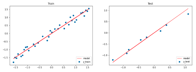
Since we only have one feature, it's easy to visually inspect the model.

# Figure size
plt.figure(figsize=(15,5))

# Plot train data
plt.subplot(1, 2, 1)
plt.title("Train")
plt.scatter(X_train, y_train, label="y_train")
plt.plot(X_train, pred_train.detach().numpy(), color="red", linewidth=1, linestyle="-", label="model")
plt.legend(loc="lower right")

# Plot test data
plt.subplot(1, 2, 2)
plt.title("Test")
plt.scatter(X_test, y_test, label='y_test')
plt.plot(X_test, pred_test.detach().numpy(), color="red", linewidth=1, linestyle="-", label="model")
plt.legend(loc="lower right")

# Show plots
plt.show()

Inference

After training a model, we can use it to predict on new data.

# Feed in your own inputs
sample_indices = [10, 15, 25]
X_infer = np.array(sample_indices, dtype=np.float32)
X_infer = torch.Tensor(X_scaler.transform(X_infer.reshape(-1, 1)))

Recall that we need to unstandardize our predictions.

\[ \hat{y}_{scaled} = \frac{\hat{y} - \mu_{\hat{y}}}{\sigma_{\hat{y}}} \]

\[ \hat{y} = \hat{y}_{scaled} * \sigma_{\hat{y}} + \mu_{\hat{y}} \]

# Unstandardize predictions
pred_infer = model(X_infer).detach().numpy() * np.sqrt(y_scaler.var_) + y_scaler.mean_
for i, index in enumerate(sample_indices):
    print (f"{df.iloc[index]["y"]:.2f} (actual) → {pred_infer[i][0]:.2f} (predicted)")

35.73 (actual) → 42.11 (predicted)
59.34 (actual) → 59.17 (predicted)
97.04 (actual) → 93.30 (predicted)

Interpretability

Linear regression offers the great advantage of being highly interpretable. Each feature has a coefficient which signifies its importance/impact on the output variable y. We can interpret our coefficient as follows: by increasing X by 1 unit, we increase y by \(W\) (~3.65) units.

# Unstandardize coefficients
W = model.fc1.weight.data.numpy()[0][0]
b = model.fc1.bias.data.numpy()[0]
W_unscaled = W * (y_scaler.scale_/X_scaler.scale_)
b_unscaled = b * y_scaler.scale_ + y_scaler.mean_ - np.sum(W_unscaled*X_scaler.mean_)
print ("[actual] y = 3.5X + noise")
print (f"[model] y_hat = {W_unscaled[0]:.1f}X + {b_unscaled[0]:.1f}")

[actual] y = 3.5X + noise
[model] y_hat = 3.4X + 8.0

Regularization

Regularization helps decrease overfitting. Below is L2 regularization (ridge regression). There are many forms of regularization but they all work to reduce overfitting in our models. With L2 regularization, we are penalizing large weight values by decaying them because having large weights will lead to preferential bias with the respective inputs and we want the model to work with all the inputs and not just a select few. There are also other types of regularization like L1 (lasso regression) which is useful for creating sparse models where some feature coefficients are zeroed out, or elastic which combines L1 and L2 penalties.

Regularization is not just for linear regression. You can use it to regularize any model's weights including the ones we will look at in future lessons.

\[ J(\theta) = \frac{1}{2}\sum_{i}(X_iW - y_i)^2 + \frac{\lambda}{2}W^TW \]

\[ \frac{\partial{J}}{\partial{W}} = X (\hat{y} - y) + \lambda W \]

\[ W = W - \alpha\frac{\partial{J}}{\partial{W}} \]

Variable	Description
\(\lambda\)	regularization coefficient
\(\alpha\)	learning rate

In PyTorch, we can add L2 regularization by adjusting our optimizer. The Adam optimizer has a weight_decay parameter which to control the L2 penalty.

L2_LAMBDA = 1e-2

# Initialize model
model = LinearRegression(input_dim=INPUT_DIM, output_dim=OUTPUT_DIM)

# Optimizer (w/ L2 regularization)
optimizer = Adam(model.parameters(), lr=LEARNING_RATE, weight_decay=L2_LAMBDA)

# Training
for epoch in range(NUM_EPOCHS):
    # Forward pass
    y_pred = model(X_train)

    # Loss
    loss = loss_fn(y_pred, y_train)

    # Zero all gradients
    optimizer.zero_grad()

    # Backward pass
    loss.backward()

    # Update weights
    optimizer.step()

    if epoch%20==0:
        print (f"Epoch: {epoch} | loss: {loss:.2f}")

Epoch: 0 | loss: 2.20
Epoch: 20 | loss: 0.06
Epoch: 40 | loss: 0.03
Epoch: 60 | loss: 0.02
Epoch: 80 | loss: 0.02

# Predictions
pred_train = model(X_train)
pred_test = model(X_test)

# Performance
train_error = loss_fn(pred_train, y_train)
test_error = loss_fn(pred_test, y_test)
print(f"train_error: {train_error:.2f}")
print(f"test_error: {test_error:.2f}")

train_error: 0.02
test_error: 0.01

Regularization didn't make a difference in performance with this specific example because our data is generated from a perfect linear equation but for large realistic data, regularization can help our model generalize well.

---

To cite this content, please use:

@article{madewithml,
    author       = {Goku Mohandas},
    title        = { Linear regression - Made With ML },
    howpublished = {\url{https://madewithml.com/}},
    year         = {2023}
}