Experiment Tracking
Repository · Notebook

Subscribe to our newsletter
📬 Receive new lessons straight to your inbox (once a month) and join 40K+ developers in learning how to responsibly deliver value with ML.
Intuition
So far, we've been training and evaluating our different baselines but haven't really been tracking these experiments. We'll fix this but defining a proper process for experiment tracking which we'll use for all future experiments (including hyperparameter optimization). Experiment tracking is the process of managing all the different experiments and their components, such as parameters, metrics, models and other artifacts and it enables us to:
- Organize all the necessary components of a specific experiment. It's important to have everything in one place and know where it is so you can use them later.
- Reproduce past results (easily) using saved experiments.
- Log iterative improvements across time, data, ideas, teams, etc.
Tools
There are many options for experiment tracking but we're going to use MLFlow (100% free and open-source) because it has all the functionality we'll need. We can run MLFlow on our own servers and databases so there are no storage cost / limitations, making it one of the most popular options and is used by Microsoft, Facebook, Databricks and others. There are also several popular options such as a Comet ML (used by Google AI, HuggingFace, etc.), Neptune (used by Roche, NewYorker, etc.), Weights and Biases (used by Open AI, Toyota Research, etc.). These are fully managed solutions that provide features like dashboards, reports, etc.
Setup
We'll start by setting up our model registry where all of our experiments and their artifacts will be stores.
1 2 3 4 | |
1 2 3 4 5 6 | |
file:///tmp/mlflow
On Windows, the tracking URI should have three forwards slashes:
1MLFLOW_TRACKING_URI = "file:///" + str(MODEL_REGISTRY.absolute())
Note
In this course, our MLflow artifact and backend store will both be on our local machine. In a production setting, these would be remote such as S3 for the artifact store and a database service (ex. PostgreSQL RDS) as our backend store.
Integration
While we could use MLflow directly to log metrics, artifacts and parameters:
1 2 3 4 | |
We'll instead use Ray to integrate with MLflow. Specifically we'll use the MLflowLoggerCallback which will automatically log all the necessary components of our experiments to the location specified in our MLFLOW_TRACKING_URI. We of course can still use MLflow directly if we want to log something that's not automatically logged by the callback. And if we're using other experiment trackers, Ray has integrations for those as well.
1 2 3 4 5 6 | |
Once we have the callback defined, all we have to do is update our RunConfig to include it.
1 2 3 4 5 | |
Training
With our updated RunConfig, with the MLflow callback, we can now train our model and all the necessary components will be logged to MLflow. This is the exact same training workflow we've been using so far from the training lesson.
1 2 3 4 5 6 7 8 9 10 11 12 13 14 15 16 17 18 19 20 21 22 23 24 | |
1 | |
We're going to use the search_runs function from the MLflow python API to identify the best run in our experiment so far (we' only done one run so far so it will be the run from above).
1 2 3 | |
run_id                                                           8e473b640d264808a89914e8068587fb
experiment_id                                                                  853333311265913081
status                                                                                   FINISHED
...
tags.mlflow.runName                                                      TorchTrainer_077f9_00000
Name: 0, dtype: object
Dashboard
Once we're done training, we can use the MLflow dashboard to visualize our results. To do so, we'll use the mlflow server command to launch the MLflow dashboard and navigate to the experiment we just created.
mlflow server -h 0.0.0.0 -p 8080 --backend-store-uri /tmp/mlflow/
View the dashboard
If you're on Anyscale Workspaces, then we need to first expose the port of the MLflow server. Run the following command on your Anyscale Workspace terminal to generate the public URL to your MLflow server.
APP_PORT=8080
echo https://$APP_PORT-port-$ANYSCALE_SESSION_DOMAIN
If you're running this notebook on your local laptop then head on over to http://localhost:8080/ to view your MLflow dashboard.
MLFlow creates a main dashboard with all your experiments and their respective runs. We can sort runs by clicking on the column headers.
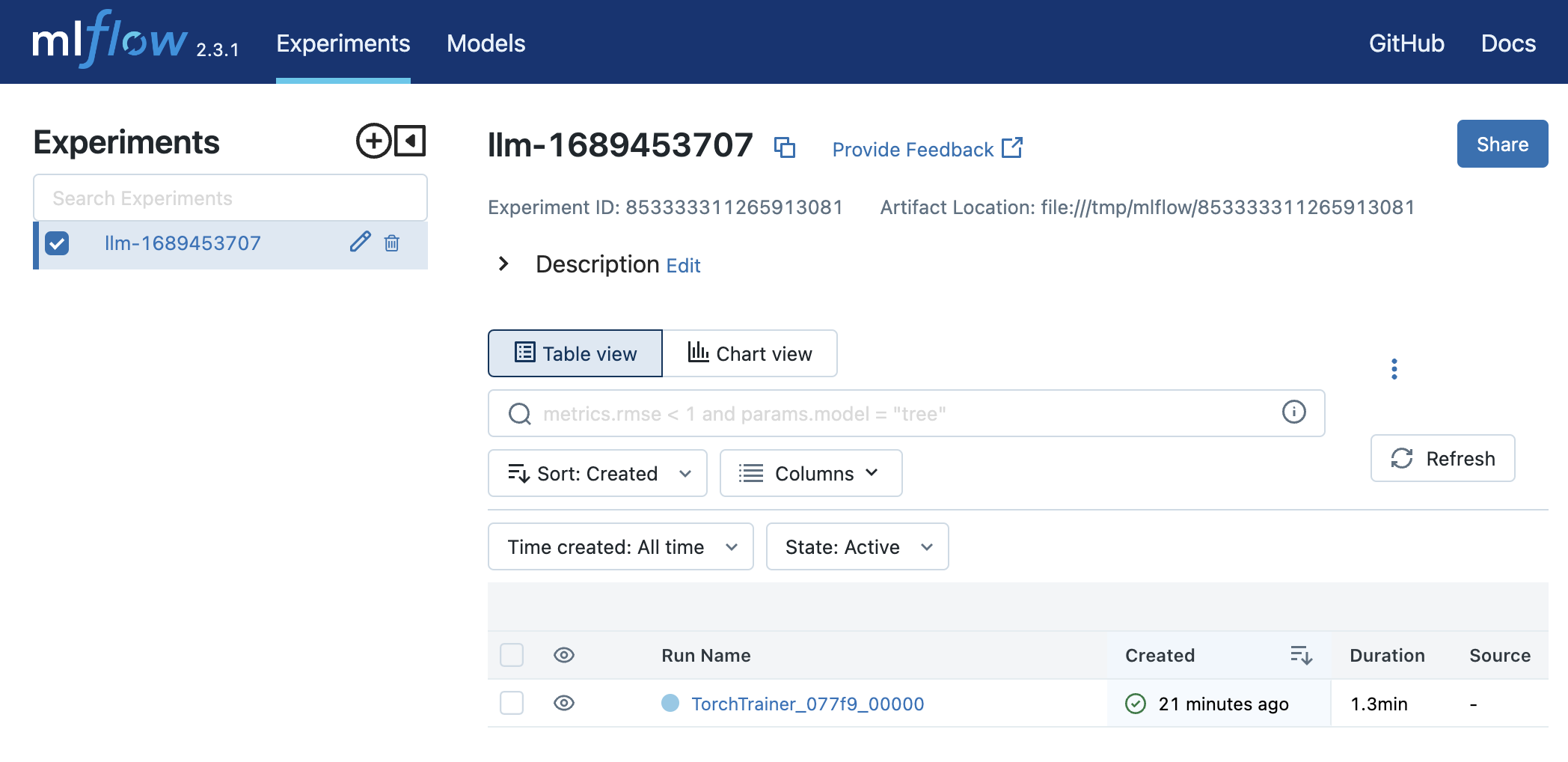
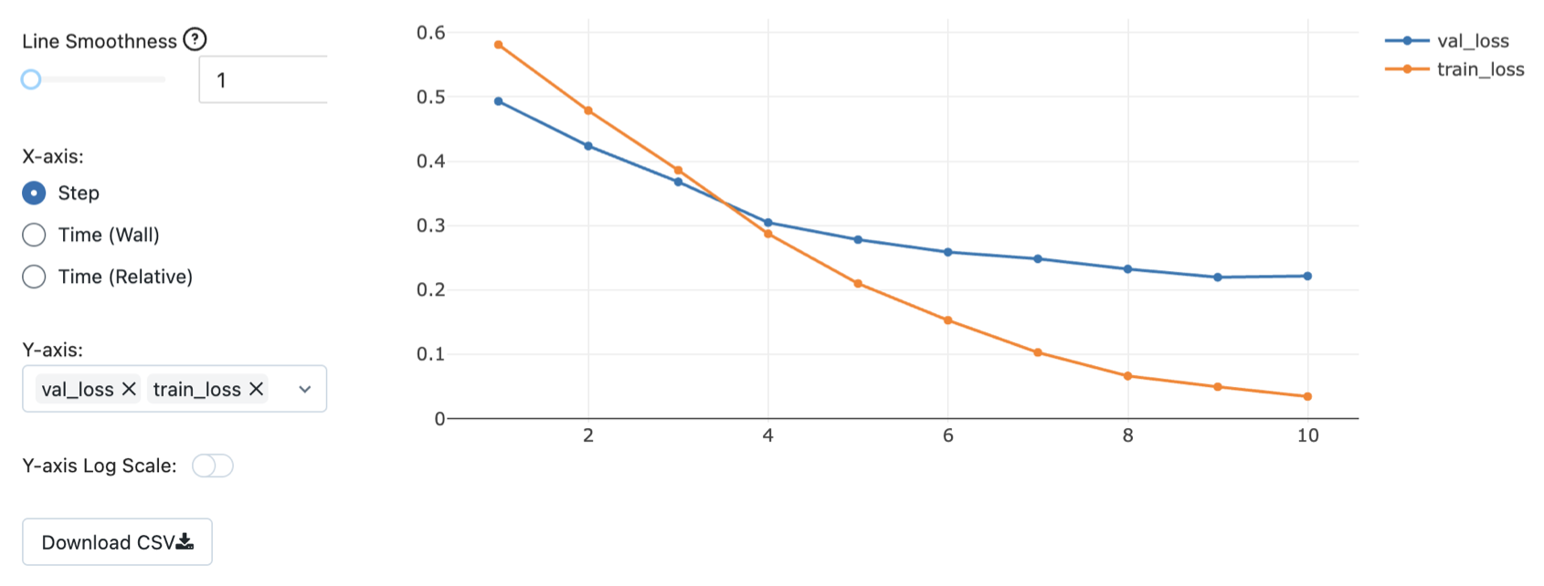
And within each run, we can view metrics, parameters, artifacts, etc.

And we can even create custom plots to help us visualize our results.
Loading
After inspection and once we've identified an experiment that we like, we can load the model for evaluation and inference.
1 2 | |
We're going to create a small utility function that uses an MLflow run's artifact path to load a Ray Result object. We'll then use the Result object to load the best checkpoint.
1 2 3 4 | |
With a particular run's best checkpoint, we can load the model from it and use it.
1 2 3 4 5 | |
{
  "precision": 0.9281010510531216,
  "recall": 0.9267015706806283,
  "f1": 0.9269438615952555
}
Before we can use our model for inference, we need to load the preprocessor from our predictor and apply it to our input data.
1 2 | |
1 2 3 4 5 | |
[{'prediction': 'natural-language-processing',
  'probabilities': {'computer-vision': 0.00038025028,
   'mlops': 0.00038209034,
   'natural-language-processing': 0.998792,
   'other': 0.00044562898}}]
In the next lesson we'll learn how to tune our models and use our MLflow dashboard to compare the results.
Upcoming live cohorts
Sign up for our upcoming live cohort, where we'll provide live lessons + QA, compute (GPUs) and community to learn everything in one day.
To cite this content, please use:
1 2 3 4 5 6 | |