📬 Receive new lessons straight to your inbox (once a month) and join 40K+
developers in learning how to responsibly deliver value with ML.
Overview
Logistic regression is an extension on linear regression (both are generalized linear methods). We will still learn to model a line (plane) that models \(y\) given \(X\). Except now we are dealing with classification problems as opposed to regression problems so we'll be predicting probability distributions as opposed to discrete values. We'll be using the softmax operation to normalize our logits (\(XW\)) to derive probabilities.
Our goal is to learn a logistic model \(\hat{y}\) that models \(y\) given \(X\).
\[ \hat{y} = \frac{e^{XW_y}}{\sum_j e^{XW}} \]
Variable
Description
\(N\)
total numbers of samples
\(C\)
number of classes
\(\hat{y}\)
predictions \(\in \mathbb{R}^{NXC}\)
\(X\)
inputs \(\in \mathbb{R}^{NXD}\)
\(W\)
weights \(\in \mathbb{R}^{DXC}\)
(*) bias term (\(b\)) excluded to avoid crowding the notations
This function is known as the multinomial logistic regression or the softmax classifier. The softmax classifier will use the linear equation (\(z=XW\)) and normalize it (using the softmax function) to produce the probability for class y given the inputs.
Objectives:
Predict the probability of class \(y\) given the inputs \(X\). The softmax classifier normalizes the linear outputs to determine class probabilities.
Advantages:
Can predict class probabilities given a set on inputs.
Disadvantages:
Sensitive to outliers since objective is to minimize cross entropy loss. Support vector machines (SVMs) are a good alternative to counter outliers.
Miscellaneous:
Softmax classifier is widely in neural network architectures as the last layer since it produces class probabilities.
Set up
We'll set our seeds for reproducibility.
12
importnumpyasnpimportrandom
1
SEED=1234
123
# Set seed for reproducibilitynp.random.seed(SEED)random.seed(SEED)
Load data
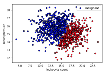
We'll used some synthesized data to train our models on. The task is to determine whether a tumor will be benign (harmless) or malignant (harmful) based on leukocyte (white blood cells) count and blood pressure. Note that this is a synthetic dataset that has no clinical relevance.
# Set seed for reproducibilitynp.random.seed(SEED)
12345
# Read from CSV to Pandas DataFrameurl="https://raw.githubusercontent.com/GokuMohandas/Made-With-ML/main/datasets/tumors.csv"df=pd.read_csv(url,header=0)# loaddf=df.sample(frac=1).reset_index(drop=True)# shuffledf.head()
leukocyte_count
blood_pressure
tumor_class
0
15.335860
14.637535
benign
1
9.857535
14.518942
malignant
2
17.632579
15.869585
benign
3
18.369174
14.774547
benign
4
14.509367
15.892224
malignant
123
# Define X and yX=df[["leukocyte_count","blood_pressure"]].valuesy=df["tumor_class"].values
We want to split our dataset so that each of the three splits has the same distribution of classes so that we can train and evaluate properly. We can easily achieve this by telling scikit-learn's train_test_split function what to stratify on.
deftrain_val_test_split(X,y,train_size):"""Split dataset into data splits."""X_train,X_,y_train,y_=train_test_split(X,y,train_size=TRAIN_SIZE,stratify=y)X_val,X_test,y_val,y_test=train_test_split(X_,y_,train_size=0.5,stratify=y_)returnX_train,X_val,X_test,y_train,y_val,y_test
# Per data split class distributiontrain_class_counts=dict(collections.Counter(y_train))val_class_counts=dict(collections.Counter(y_val))test_class_counts=dict(collections.Counter(y_test))print(f'train m:b = {train_class_counts["malignant"]/train_class_counts["benign"]:.2f}')print(f'val m:b = {val_class_counts["malignant"]/val_class_counts["benign"]:.2f}')print(f'test m:b = {test_class_counts["malignant"]/test_class_counts["benign"]:.2f}')
train m:b = 1.57
val m:b = 1.54
test m:b = 1.59
Label encoding
You'll notice that our class labels are text. We need to encode them into integers so we can use them in our models. We could scikit-learn's LabelEncoder to do this but we're going to write our own simple label encoder class so we can see what's happening under the hood.
classLabelEncoder(object):"""Label encoder for tag labels."""def__init__(self,class_to_index={}):self.class_to_index=class_to_indexor{}# mutable defaults ;)self.index_to_class={v:kfork,vinself.class_to_index.items()}self.classes=list(self.class_to_index.keys())def__len__(self):returnlen(self.class_to_index)def__str__(self):returnf"<LabelEncoder(num_classes={len(self)})>"deffit(self,y):classes=np.unique(y)fori,class_inenumerate(classes):self.class_to_index[class_]=iself.index_to_class={v:kfork,vinself.class_to_index.items()}self.classes=list(self.class_to_index.keys())returnselfdefencode(self,y):encoded=np.zeros((len(y)),dtype=int)fori,iteminenumerate(y):encoded[i]=self.class_to_index[item]returnencodeddefdecode(self,y):classes=[]fori,iteminenumerate(y):classes.append(self.index_to_class[item])returnclassesdefsave(self,fp):withopen(fp,"w")asfp:contents={'class_to_index':self.class_to_index}json.dump(contents,fp,indent=4,sort_keys=False)@classmethoddefload(cls,fp):withopen(fp,"r")asfp:kwargs=json.load(fp=fp)returncls(**kwargs)
We also want to calculate our class weights, which are useful for weighting the loss function during training. It tells the model to focus on samples from an under-represented class. The loss section below will show how to incorporate these weights.
1234
# Class weightscounts=np.bincount(y_train)class_weights={i:1.0/countfori,countinenumerate(counts)}print(f"counts: {counts}\nweights: {class_weights}")
We need to standardize our data (zero mean and unit variance) so a specific feature's magnitude doesn't affect how the model learns its weights. We're only going to standardize the inputs X because our outputs y are class values.
1
fromsklearn.preprocessingimportStandardScaler
12
# Standardize the data (mean=0, std=1) using training dataX_scaler=StandardScaler().fit(X_train)
1234
# Apply scaler on training and test data (don't standardize outputs for classification)X_train=X_scaler.transform(X_train)X_val=X_scaler.transform(X_val)X_test=X_scaler.transform(X_test)
123
# Check (means should be ~0 and std should be ~1)print(f"X_test[0]: mean: {np.mean(X_test[:,0],axis=0):.1f}, std: {np.std(X_test[:,0],axis=0):.1f}")print(f"X_test[1]: mean: {np.mean(X_test[:,1],axis=0):.1f}, std: {np.std(X_test[:,1],axis=0):.1f}")
Now that we have our data prepared, we'll first implement logistic regression using just NumPy. This will let us really understand the underlying operations. It's normal to find the math and code in this section slightly complex. You can still read each of the steps to build intuition for when we implement this using PyTorch.
Our goal is to learn a logistic model \(\hat{y}\) that models \(y\) given \(X\).
\[ \hat{y} = \frac{e^{XW_y}}{\sum_j e^{XW}} \]
We are going to use multinomial logistic regression even though our task only involves two classes because you can generalize the softmax classifier to any number of classes.
Initialize weights
Step 1: Randomly initialize the model's weights \(W\).
12
INPUT_DIM=X_train.shape[1]# X is 2-dimensionalNUM_CLASSES=len(label_encoder.classes)# y has two possibilities (benign or malignant)
12345
# Initialize random weightsW=0.01*np.random.randn(INPUT_DIM,NUM_CLASSES)b=np.zeros((1,NUM_CLASSES))print(f"W: {W.shape}")print(f"b: {b.shape}")
W: (2, 2)
b: (1, 2)
Model
Step 2: Feed inputs \(X\) into the model to receive the logits (\(z=XW\)). Apply the softmax operation on the logits to get the class probabilities \(\hat{y}\) in one-hot encoded form. For example, if there are three classes, the predicted class probabilities could look like [0.3, 0.3, 0.4].
# Normalization via softmax to obtain class probabilitiesexp_logits=np.exp(logits)y_hat=exp_logits/np.sum(exp_logits,axis=1,keepdims=True)print(f"y_hat: {y_hat.shape}")print(f"sample: {y_hat[0]}")
y_hat: (722, 2)
sample: [0.50295525 0.49704475]
Loss
Step 3: Compare the predictions \(\hat{y}\) (ex. [0.3, 0.3, 0.4]) with the actual target values \(y\) (ex. class 2 would look like [0, 0, 1]) with the objective (cost) function to determine loss \(J\). A common objective function for logistics regression is cross-entropy loss.
Step 4: Calculate the gradient of loss \(J(\theta)\) w.r.t to the model weights. Let's assume that our classes are mutually exclusive (a set of inputs could only belong to one class).
Step 5: Update the weights \(W\) using a small learning rate \(\alpha\). The updates will penalize the probability for the incorrect classes (j) and encourage a higher probability for the correct class (y).
# Training and test accuracytrain_acc=np.mean(np.equal(y_train,pred_train))test_acc=np.mean(np.equal(y_test,pred_test))print(f"train acc: {train_acc:.2f}, test acc: {test_acc:.2f}")
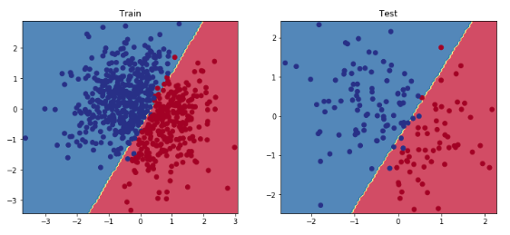
defplot_multiclass_decision_boundary(model,X,y,savefig_fp=None):"""Plot the multiclass decision boundary for a model that accepts 2D inputs. Credit: https://cs231n.github.io/neural-networks-case-study/ Arguments: model {function} -- trained model with function model.predict(x_in). X {numpy.ndarray} -- 2D inputs with shape (N, 2). y {numpy.ndarray} -- 1D outputs with shape (N,). """# Axis boundariesx_min,x_max=X[:,0].min()-0.1,X[:,0].max()+0.1y_min,y_max=X[:,1].min()-0.1,X[:,1].max()+0.1xx,yy=np.meshgrid(np.linspace(x_min,x_max,101),np.linspace(y_min,y_max,101))# Create predictionsx_in=np.c_[xx.ravel(),yy.ravel()]y_pred=model.predict(x_in)y_pred=np.argmax(y_pred,axis=1).reshape(xx.shape)# Plot decision boundaryplt.contourf(xx,yy,y_pred,cmap=plt.cm.Spectral,alpha=0.8)plt.scatter(X[:,0],X[:,1],c=y,s=40,cmap=plt.cm.RdYlBu)plt.xlim(xx.min(),xx.max())plt.ylim(yy.min(),yy.max())# Plotifsavefig_fp:plt.savefig(savefig_fp,format="png")
123456789
# Visualize the decision boundaryplt.figure(figsize=(12,5))plt.subplot(1,2,1)plt.title("Train")plot_multiclass_decision_boundary(model=model,X=X_train,y=y_train)plt.subplot(1,2,2)plt.title("Test")plot_multiclass_decision_boundary(model=model,X=X_test,y=y_test)plt.show()
PyTorch
Now that we've implemented logistic regression with Numpy, let's do the same with PyTorch.
1
importtorch
12
# Set seed for reproducibilitytorch.manual_seed(SEED)
Model
We will be using PyTorch's Linear layers to recreate the same model.
We'll compute accuracy as we train our model because just looking the loss value isn't super intuitive to look at. We'll look at other metrics (precision, recall, f1) in the evaluation section below.
# Convert data to tensorsX_train=torch.Tensor(X_train)y_train=torch.LongTensor(y_train)X_val=torch.Tensor(X_val)y_val=torch.LongTensor(y_val)X_test=torch.Tensor(X_test)y_test=torch.LongTensor(y_test)
1 2 3 4 5 6 7 8 9101112131415161718192021
# Trainingforepochinrange(NUM_EPOCHS):# Forward passy_pred=model(X_train)# Lossloss=loss_fn(y_pred,y_train)# Zero all gradientsoptimizer.zero_grad()# Backward passloss.backward()# Update weightsoptimizer.step()ifepoch%10==0:predictions=y_pred.max(dim=1)[1]# classaccuracy=accuracy_fn(y_pred=predictions,y_true=y_train)print(f"Epoch: {epoch} | loss: {loss:.2f}, accuracy: {accuracy:.1f}")
# Accuracy (could've also used our own accuracy function)train_acc=accuracy_score(y_train,pred_train)test_acc=accuracy_score(y_test,pred_test)print(f"train acc: {train_acc:.2f}, test acc: {test_acc:.2f}")
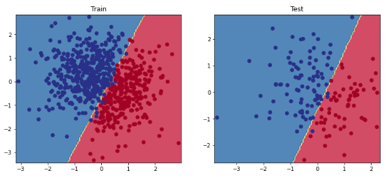
train acc: 0.98, test acc: 0.98
We can also evaluate our model on other meaningful metrics such as precision and recall. These are especially useful when there is data imbalance present.
# Visualize the decision boundaryplt.figure(figsize=(12,5))plt.subplot(1,2,1)plt.title("Train")plot_multiclass_decision_boundary(model=model,X=X_train,y=y_train)plt.subplot(1,2,2)plt.title("Test")plot_multiclass_decision_boundary(model=model,X=X_test,y=y_test)plt.show()
Inference
12
# Inputs for inferenceX_infer=pd.DataFrame([{"leukocyte_count":13,"blood_pressure":12}])
# Predicty_infer=F.softmax(model(torch.Tensor(X_infer)),dim=1)prob,_class=y_infer.max(dim=1)label=label_encoder.decode(_class.detach().numpy())[0]print(f"The probability that you have a {label} tumor is {prob.detach().numpy()[0]*100.0:.0f}%")
The probability that you have a benign tumor is 93%