📬 Receive new lessons straight to your inbox (once a month) and join 40K+
developers in learning how to responsibly deliver value with ML.
Intuition
Hyperparameter tuning is the process of discovering a set of performant parameter values for our model. It can be a computationally involved process depending on the number of parameters, search space and model architectures. Hyperparameters don't just include the model's parameters but could also include parameters related to preprocessing, splitting, etc. When we look at all the different parameters that can be tuned, it quickly becomes a very large search space. However, just because something is a hyperparameter doesn't mean we need to tune it.
It's absolutely acceptable to fix some hyperparameters (ex. using lower cased text [lower=True] during preprocessing).
You can initially just tune a small, yet influential, subset of hyperparameters that you believe will yield great results.
We want to optimize our hyperparameters so that we can understand how each of them affects our objective. By running many trials across a reasonable search space, we can determine near ideal values for our different parameters.
Frameworks
There are many options for hyperparameter tuning (Ray tune, Optuna, Hyperopt, etc.). We'll be using Ray Tune with it's HyperOpt integration for it's simplicity and general popularity. Ray Tune also has a wide variety of support for many other tune search algorithms (Optuna, Bayesian, etc.).
Set up
There are many factors to consider when performing hyperparameter tuning. We'll be conducting a small study where we'll tune just a few key hyperparameters across a few trials. Feel free to include additional parameters and to increase the number trials in the tuning experiment.
12
# Number of trials (small sample)num_runs=2
We'll start with some the set up, data and model prep as we've done in previous lessons.
We can think of tuning as training across different combinations of parameters. For this, we'll need to define several configurations around when to stop tuning (stopping criteria), how to define the next set of parameters to train with (search algorithm) and even the different values that the parameters can take (search space).
# Run configurationcheckpoint_config=CheckpointConfig(num_to_keep=1,checkpoint_score_attribute="val_loss",checkpoint_score_order="min")run_config=RunConfig(callbacks=[mlflow_callback],checkpoint_config=checkpoint_config)
Notice that we use the same mlflow_callback from our experiment tracking lesson so all of our runs will be tracked to MLflow automatically.
Search algorithm
Next, we're going to set the initial parameter values and the search algorithm (HyperOptSearch) for our tuning experiment. We're also going to set the maximum number of trials that can be run concurrently (ConcurrencyLimiter) based on the compute resources we have.
1234
# Hyperparameters to start withinitial_params=[{"train_loop_config":{"dropout_p":0.5,"lr":1e-4,"lr_factor":0.8,"lr_patience":3}}]search_alg=HyperOptSearch(points_to_evaluate=initial_params)search_alg=ConcurrencyLimiter(search_alg,max_concurrent=2)
Tip
It's a good idea to start with some initial parameter values that you think might be reasonable. This can help speed up the tuning process and also guarantee at least one experiment that will perform decently well.
Search space
Next, we're going to define the parameter search space by choosing the parameters, their distribution and range of values. Depending on the parameter type, we have many different distributions to choose from.
Next, we're going to define a scheduler to prune unpromising trials. We'll be using AsyncHyperBandScheduler (ASHA), which is a very popular and aggressive early-stopping algorithm. Due to our aggressive scheduler, we'll set a grace_period to allow the trials to run for at least a few epochs before pruning and a maximum of max_t epochs.
12345
# Schedulerscheduler=AsyncHyperBandScheduler(max_t=train_loop_config["num_epochs"],# max epoch (<time_attr>) per trialgrace_period=5,# min epoch (<time_attr>) per trial)
Tuner
Finally, we're going to define a TuneConfig that will combine the search_alg and scheduler we've defined above.
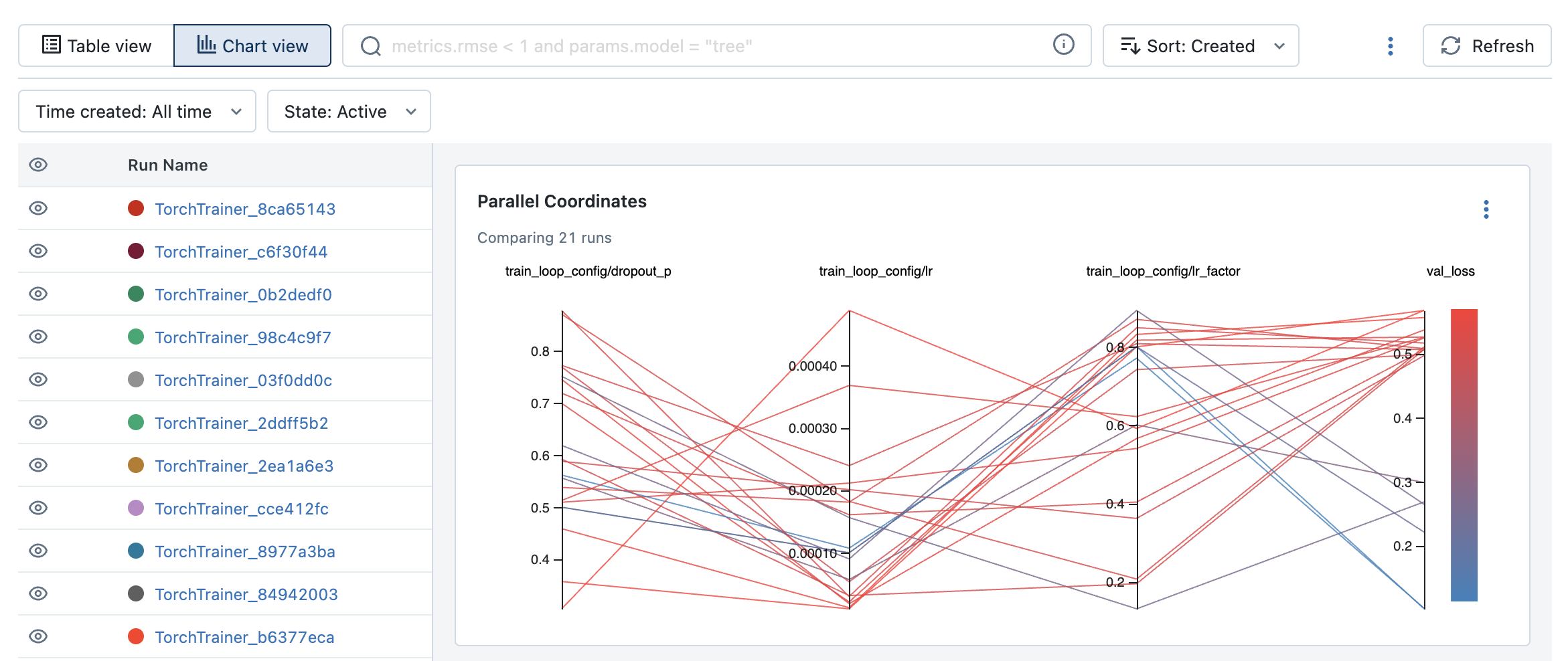
And on our MLflow dashboard, we can create useful plots like a parallel coordinates plot to visualize the different hyperparameters and their values across the different trials.
Best trial
And from these results, we can extract the best trial and its hyperparameters:
123
# Best trial's epochsbest_trial=results.get_best_result(metric="val_loss",mode="min")best_trial.metrics_dataframe
epoch
lr
train_loss
val_loss
timestamp
time_this_iter_s
should_checkpoint
done
training_iteration
trial_id
date
time_total_s
pid
hostname
node_ip
time_since_restore
iterations_since_restore
0
0
0.0001
0.582092
0.495889
1689460489
14.537316
True
False
1
094e2a7e
2023-07-15_15-34-53
14.537316
94006
ip-10-0-48-210
10.0.48.210
14.537316
1
1
1
0.0001
0.492427
0.430734
1689460497
7.144841
True
False
2
094e2a7e
2023-07-15_15-35-00
21.682157
94006
ip-10-0-48-210
10.0.48.210
21.682157
2
...
...
...
...
...
...
...
...
...
...
...
...
...
...
...
...
...
...
9
9
0.0001
0.040960
0.217990
1689460552
6.890944
True
True
10
094e2a7e
2023-07-15_15-35-55
76.588228
94006
ip-10-0-48-210
10.0.48.210
76.588228
10
12
# Best trial's hyperparametersbest_trial.config["train_loop_config"]
From this we can load the best checkpoint from the best run and evaluate it on the test split.
123456
# Evaluate on test splitrun_id=sorted_runs.iloc[0].run_idbest_checkpoint=get_best_checkpoint(run_id=run_id)predictor=TorchPredictor.from_checkpoint(best_checkpoint)performance=evaluate(ds=test_ds,predictor=predictor)print(json.dumps(performance,indent=2))
# Predict on sampletitle="Transfer learning with transformers"description="Using transformers for transfer learning on text classification tasks."sample_df=pd.DataFrame([{"title":title,"description":description,"tag":"other"}])predict_with_proba(df=sample_df,predictor=predictor)
Now that we're tuned our model, in the next lesson, we're going to perform a much more intensive evaluation on our model compared to just viewing it's overall metrics on a test set.
Upcoming live cohorts
Sign up for our upcoming live cohort, where we'll provide live lessons + QA, compute (GPUs) and community to learn everything in one day.
To cite this content, please use:
123456
@article{madewithml,author={Goku Mohandas},title={ Tuning - Made With ML },howpublished={\url{https://madewithml.com/}},year={2023}}