NumPy for Machine Learning
Repository · Notebook
Subscribe to our newsletter
📬 Receive new lessons straight to your inbox (once a month) and join 40K+ developers in learning how to responsibly deliver value with ML.
Set up
First we'll import the NumPy package and set seeds for reproducibility so that we can receive the exact same results every time.
1 | |
1 2 | |
Basics
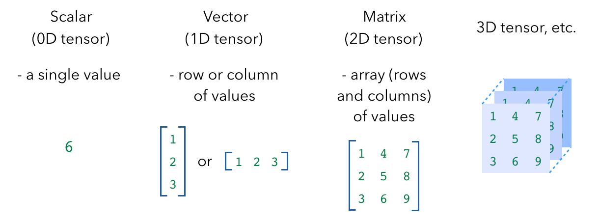
1 2 3 4 5 6 7 | |
x:  6
x ndim:  0
x shape: ()
x size:  1
x dtype:  int64
1 2 3 4 5 6 7 | |
x:  [1.3 2.2 1.7]
x ndim:  1
x shape: (3,)
x size:  3
x dtype:  float64
1 2 3 4 5 6 7 | |
x:
 [[1 2]
 [3 4]]
x ndim:  2
x shape: (2, 2)
x size:  4
x dtype:  int64
1 2 3 4 5 6 7 | |
x:
 [[[1 2]
  [3 4]]

 [[5 6]
  [7 8]]]
x ndim:  3
x shape: (2, 2, 2)
x size:  8
x dtype:  int64
NumPy also comes with several functions that allow us to create tensors quickly.
1 2 3 4 5 | |
np.zeros((2,2)):
 [[0. 0.]
 [0. 0.]]
np.ones((2,2)):
 [[1. 1.]
 [1. 1.]]
np.eye((2)):
 [[1. 0.]
 [0. 1.]]
np.random.random((2,2)):
 [[0.19151945 0.62210877]
 [0.43772774 0.78535858]]
Indexing
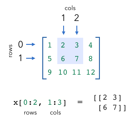
We can extract specific values from our tensors using indexing.
Keep in mind that when indexing the row and column, indices start at
0. And like indexing with lists, we can use negative indices as well (where-1is the last item).
1 2 3 4 5 6 | |
x:  [1 2 3]
x[0]:  1
x:  [0 2 3]
1 2 3 4 5 6 | |
[[ 1  2  3  4]
 [ 5  6  7  8]
 [ 9 10 11 12]]
x column 1:  [ 2  6 10]
x row 0:  [1 2 3 4]
x rows 0,1 & cols 1,2:
 [[2 3]
 [6 7]]
1 2 3 4 5 6 7 8 | |
[[ 1  2  3  4]
 [ 5  6  7  8]
 [ 9 10 11 12]]
rows_to_get:  [0 1 2]
cols_to_get:  [0 2 1]
indexed values:  [ 1  7 10]
1 2 3 4 5 | |
x:
 [[1 2]
 [3 4]
 [5 6]]
x > 2:
 [[False False]
 [ True  True]
 [ True  True]]
x[x > 2]:
 [3 4 5 6]
Arithmetic
1 2 3 4 5 6 | |
x + y:
 [[2. 4.]
 [6. 8.]]
x - y:
 [[0. 0.]
 [0. 0.]]
x * y:
 [[ 1.  4.]
 [ 9. 16.]]
Dot product
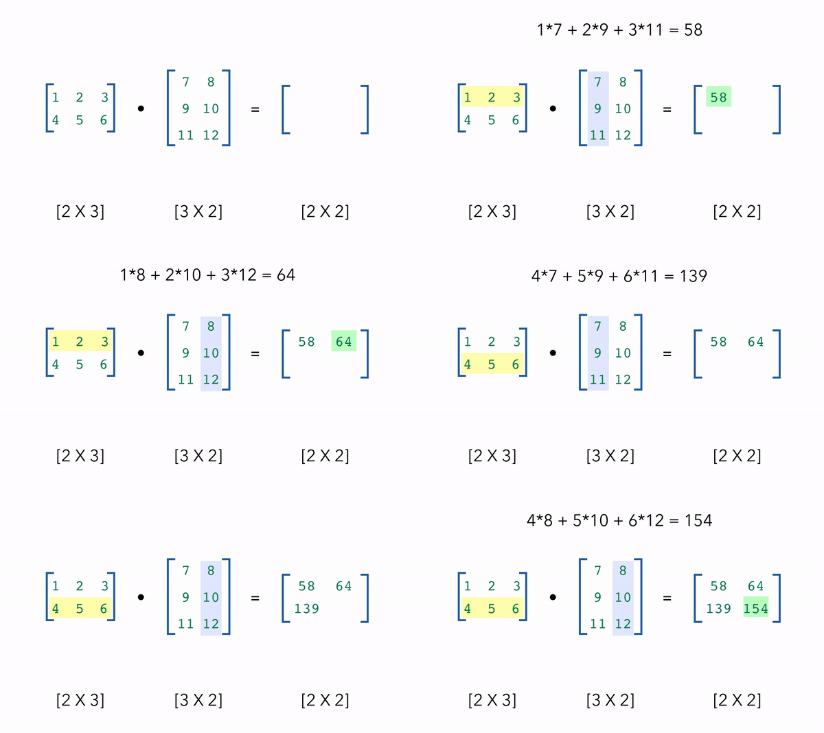
One of the most common NumPy operations we’ll use in machine learning is matrix multiplication using the dot product. Suppose we wanted to take the dot product of two matrices with shapes [2 X 3] and [3 X 2]. We take the rows of our first matrix (2) and the columns of our second matrix (2) to determine the dot product, giving us an output of [2 X 2]. The only requirement is that the inside dimensions match, in this case the first matrix has 3 columns and the second matrix has 3 rows.
1 2 3 4 5 6 | |
(2, 3) · (3, 2) = (2, 2)
[[ 58.  64.]
 [139. 154.]]
Axis operations
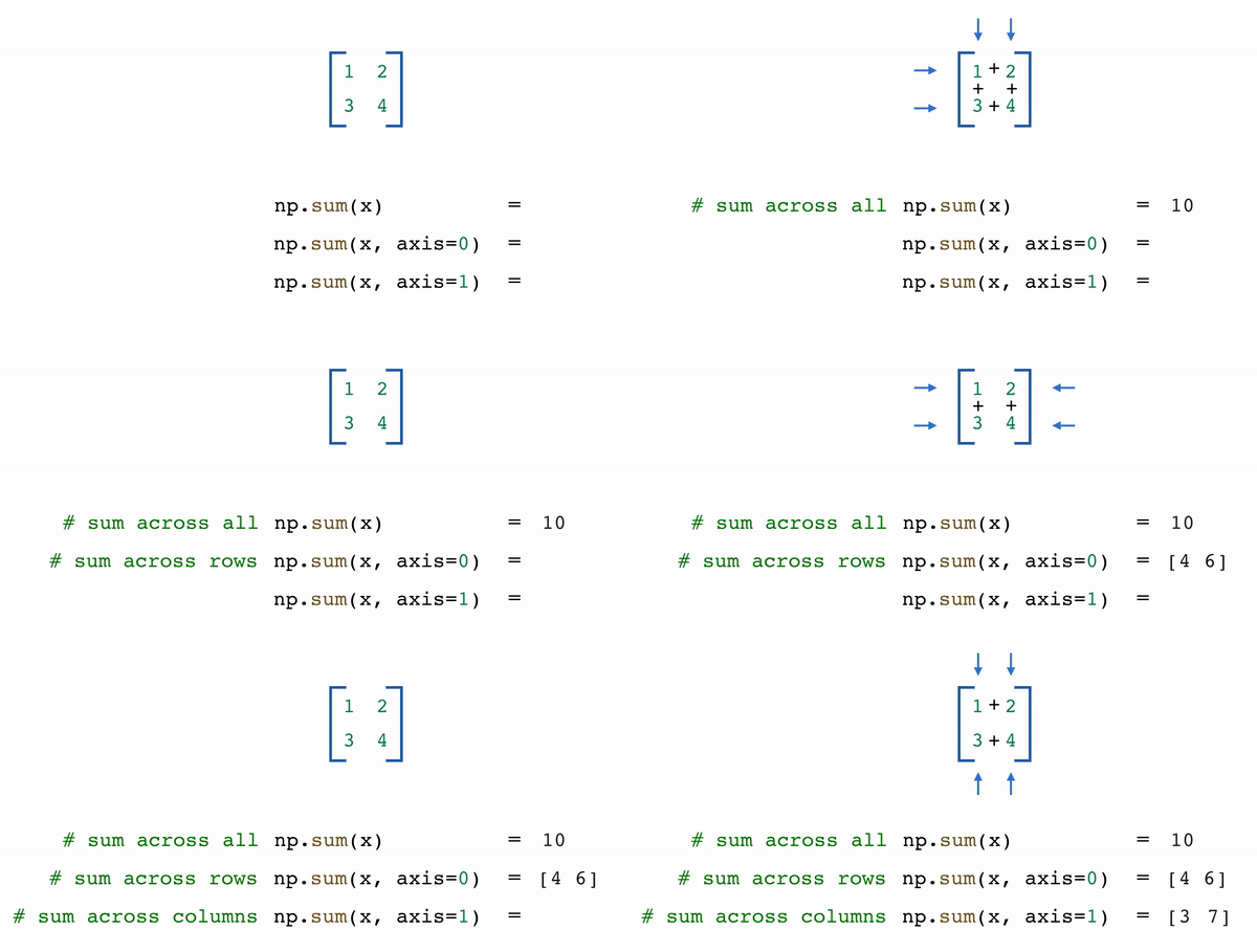
We can also do operations across a specific axis.
1 2 3 4 5 6 | |
[[1 2]
 [3 4]]
sum all:  10
sum axis=0:  [4 6]
sum axis=1:  [3 7]
1 2 3 4 5 6 | |
min:  1
max:  6
min axis=0:  [1 2 3]
min axis=1:  [1 4]
Broadcast
What happens when we try to do operations with tensors with seemingly incompatible shapes? Their dimensions aren’t compatible as is but how does NumPy still gives us the right result? This is where broadcasting comes in. The scalar is broadcast across the vector so that they have compatible shapes.
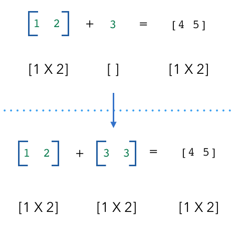
1 2 3 4 5 | |
z:
 [4 5]
Gotchas
In the situation below, what is the value of c and what are its dimensions?
1 2 3 | |
1 2 3 4 | |
array([[ 6,  7,  8],
        [ 7,  8,  9],
        [ 8,  9, 10]])
How can we fix this? We need to be careful to ensure that a is the same shape as b if we don't want this unintentional broadcasting behavior.
1 2 3 4 5 | |
array([[ 6],
       [ 8],
       [10]])
This kind of unintended broadcasting happens more often then you'd think because this is exactly what happens when we create an array from a list. So we need to ensure that we apply the proper reshaping before using it for any operations.
1 2 3 4 | |
Transpose
We often need to change the dimensions of our tensors for operations like the dot product. If we need to switch two dimensions, we can transpose the tensor.
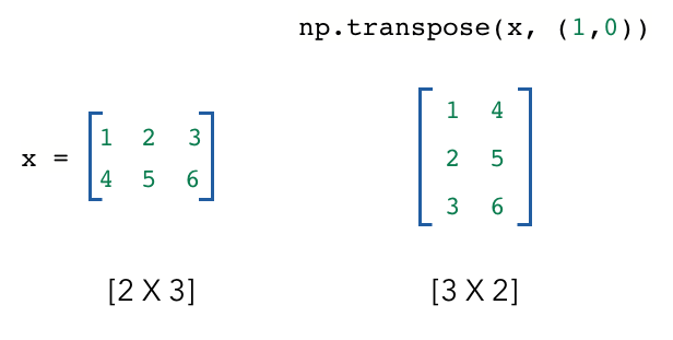
1 2 3 4 5 6 7 | |
x:
 [[1 2 3]
 [4 5 6]]
x.shape:  (2, 3)
y:
 [[1 4]
 [2 5]
 [3 6]]
y.shape:  (3, 2)
Reshape
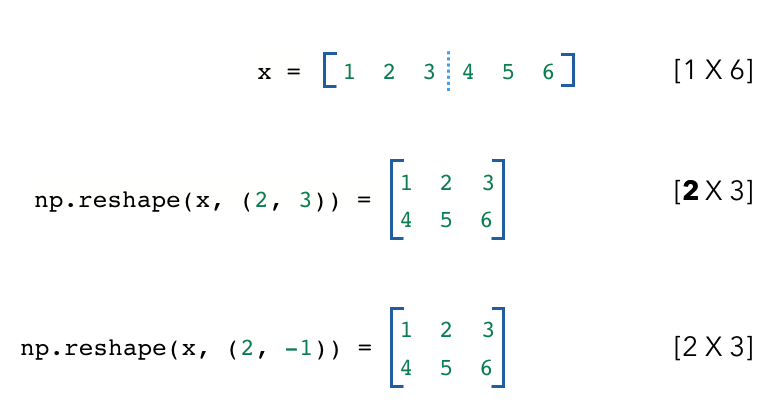
Sometimes, we'll need to alter the dimensions of the matrix. Reshaping allows us to transform a tensor into different permissible shapes. Below, our reshaped tensor has the same number of values as the original tensor. (1X6 = 2X3). We can also use -1 on a dimension and NumPy will infer the dimension based on our input tensor.
1 2 3 4 5 6 7 8 9 10 | |
[[1 2 3 4 5 6]]
x.shape:  (1, 6)
y:
 [[1 2 3]
 [4 5 6]]
y.shape:  (2, 3)
z:
 [[1 2 3]
 [4 5 6]]
z.shape:  (2, 3)
The way reshape works is by looking at each dimension of the new tensor and separating our original tensor into that many units. So here the dimension at index 0 of the new tensor is 2 so we divide our original tensor into 2 units, and each of those has 3 values.
Unintended reshaping
Though reshaping is very convenient to manipulate tensors, we must be careful of its pitfalls as well. Let's look at the example below. Suppose we have x, which has the shape [2 X 3 X 4].
1 2 3 4 | |
x: [[[ 1 1 1 1] [ 2 2 2 2] [ 3 3 3 3]][[10 10 10 10] [20 20 20 20] [30 30 30 30]]] x.shape: (2, 3, 4)
We want to reshape x so that it has shape [3 X 8] but we want the output to look like this:
[[ 1  1  1  1 10 10 10 10]
[ 2  2  2  2 20 20 20 20]
[ 3  3  3  3 30 30 30 30]]
and not like:
[[ 1  1  1  1  2  2  2  2]
[ 3  3  3  3 10 10 10 10]
[20 20 20 20 30 30 30 30]]
even though they both have the same shape [3X8]. What is the right way to reshape this?
Show answer
When we naively do a reshape, we get the right shape but the values are not what we're looking for.

1 2 3 4 | |
z_incorrect:
[[ 1  1  1  1  2  2  2  2]
[ 3  3  3  3 10 10 10 10]
[20 20 20 20 30 30 30 30]]
z_incorrect.shape:  (3, 8)
Instead, if we transpose the tensor and then do a reshape, we get our desired tensor. Transpose allows us to put our two vectors that we want to combine together and then we use reshape to join them together. And as a general rule, we should always get our dimensions together before reshaping to combine them.
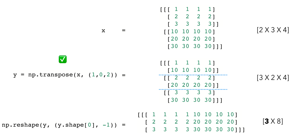
1 2 3 4 5 6 7 | |
y: [[[ 1 1 1 1] [10 10 10 10]][[ 2 2 2 2] [20 20 20 20]]
[[ 3 3 3 3] [30 30 30 30]]] y.shape: (3, 2, 4) z_correct: [[ 1 1 1 1 10 10 10 10] [ 2 2 2 2 20 20 20 20] [ 3 3 3 3 30 30 30 30]] z_correct.shape: (3, 8)
This becomes difficult when we're dealing with weight tensors with random values in many machine learning tasks. So a good idea is to always create a dummy example like this when you’re unsure about reshaping. Blindly going by the tensor shape can lead to lots of issues downstream.
Joining
We can also join our tensors via concatentation or stacking.
1 2 3 | |
[[0.79564718 0.73023418 0.92340453]
 [0.24929281 0.0513762  0.66149188]]
(2, 3)
1 2 3 4 | |
[[0.79564718 0.73023418 0.92340453]
 [0.24929281 0.0513762  0.66149188]
 [0.79564718 0.73023418 0.92340453]
 [0.24929281 0.0513762  0.66149188]]
(4, 3)
1 2 3 4 | |
[[[0.79564718 0.73023418 0.92340453]
  [0.24929281 0.0513762  0.66149188]]

 [[0.79564718 0.73023418 0.92340453]
  [0.24929281 0.0513762  0.66149188]]]
(2, 2, 3)
Expanding / reducing
We can also easily add and remove dimensions to our tensors and we'll want to do this to make tensors compatible for certain operations.
1 2 3 4 5 6 7 | |
x:
 [[1 2 3]
  [4 5 6]]
x.shape:  (2, 3)
y:
 [[[1 2 3]]
  [[4 5 6]]]
y.shape:  (2, 1, 3)
1 2 3 4 5 6 7 | |
x:
 [[[1 2 3]]
  [[4 5 6]]]
x.shape:  (2, 1, 3)
y:
 [[1 2 3]
  [4 5 6]]
y.shape:  (2, 3)
Check out Dask for scaling NumPy workflows with minimal change to existing code.
To cite this content, please use:
1 2 3 4 5 6 | |
