Evaluating Machine Learning Models
Repository · Notebook

Subscribe to our newsletter
📬 Receive new lessons straight to your inbox (once a month) and join 40K+ developers in learning how to responsibly deliver value with ML.
Intuition
Evaluation is an integral part of modeling and it's one that's often glossed over. We'll often find evaluation to involve simply computing the accuracy or other global metrics but for many real work applications, a much more nuanced evaluation process is required. However, before evaluating our model, we always want to:
- be clear about what metrics we are prioritizing
- be careful not to over optimize on any one metric because it may mean you're compromising something else
Setup
Let's start by setting up our metrics dictionary that we'll fill in as we go along and all the data we'll need for evaluation: grounds truth labels (y_test, predicted labels (y_pred) and predicted probabilities (y_prob).
1 2 | |
1 2 3 4 5 | |
1 2 3 4 | |
1 2 3 4 | |
1 2 3 4 5 | |
Coarse-grained
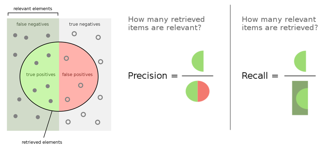
While we were developing our models, our evaluation process involved computing the coarse-grained metrics such as overall precision, recall and f1 metrics.
- True positives (TP): we correctly predicted class X.
- False positives (FP): we incorrectly predicted class X but it was another class.
- True negatives (TN): we correctly predicted that it's wasn't the class X.
- False negatives (FN): we incorrectly predicted that it wasn't the class X but it was.
1 | |
1 2 3 4 5 6 7 | |
{
    "precision": 0.916248340770615,
    "recall": 0.9109947643979057,
    "f1": 0.9110623702438432,
    "num_samples": 191.0
}
Note
The precision_recall_fscore_support() function from scikit-learn has an input parameter called average which has the following options below. We'll be using the different averaging methods for different metric granularities.
None: metrics are calculated for each unique class.binary: used for binary classification tasks where thepos_labelis specified.micro: metrics are calculated using global TP, FP, and FN.macro: per-class metrics which are averaged without accounting for class imbalance.weighted: per-class metrics which are averaged by accounting for class imbalance.samples: metrics are calculated at the per-sample level.
Fine-grained
Inspecting these coarse-grained, overall metrics is a start but we can go deeper by evaluating the same fine-grained metrics at the categorical feature levels.
1 | |
1 2 3 4 5 6 7 8 9 | |
1 2 3 | |
{
  "precision": 0.9036144578313253,
  "recall": 0.9615384615384616,
  "f1": 0.9316770186335404,
  "num_samples": 78.0
}
1 2 3 4 5 | |
[
  "natural-language-processing",
  {
    "precision": 0.9036144578313253,
    "recall": 0.9615384615384616,
    "f1": 0.9316770186335404,
    "num_samples": 78.0
  }
]
[
  "computer-vision",
  {
    "precision": 0.9838709677419355,
    "recall": 0.8591549295774648,
    "f1": 0.9172932330827067,
    "num_samples": 71.0
  }
]
[
  "other",
  {
    "precision": 0.8333333333333334,
    "recall": 0.9615384615384616,
    "f1": 0.8928571428571429,
    "num_samples": 26.0
  }
]
[
  "mlops",
  {
    "precision": 0.8125,
    "recall": 0.8125,
    "f1": 0.8125,
    "num_samples": 16.0
  }
]
Confusion matrix
Besides just inspecting the metrics for each class, we can also identify the true positives, false positives and false negatives. Each of these will give us insight about our model beyond what the metrics can provide.
- True positives (TP): learn about where our model performs well.
- False positives (FP): potentially identify samples which may need to be relabeled.
- False negatives (FN): identify the model's less performant areas to oversample later.
It's a good to have our FP/FN samples feed back into our annotation pipelines in the event we want to fix their labels and have those changes be reflected everywhere.
1 2 3 4 5 6 7 8 9 10 11 12 | |
1 2 3 | |
[4, 9, 12, 17, 19, 23, 25, 26, 29, 30, 31, 32, 33, 34, 42, 47, 49, 50, 54, 56, 65, 66, 68, 71, 75, 76, 77, 78, 79, 82, 92, 94, 95, 97, 99, 101, 109, 113, 114, 118, 120, 122, 126, 128, 129, 130, 131, 133, 134, 135, 138, 139, 140, 141, 142, 144, 148, 149, 152, 159, 160, 161, 163, 166, 170, 172, 173, 174, 177, 179, 183, 184, 187, 189, 190]
[41, 44, 73, 102, 110, 150, 154, 165]
[16, 112, 115]
1 2 3 4 5 6 7 8 9 10 | |
=== True positives ===
Mention Classifier Category prediction model
This repo contains AllenNLP model for prediction of Named Entity categories by its mentions.
    true: natural-language-processing
    pred: natural-language-processing

Finetune: Scikit-learn Style Model Finetuning for NLP Finetune is a library that allows users to leverage state-of-the-art pretrained NLP models for a wide variety of downstream tasks.
    true: natural-language-processing
    pred: natural-language-processing

Finetuning Transformers with JAX + Haiku Walking through a port of the RoBERTa pre-trained model to JAX + Haiku, then fine-tuning the model to solve a downstream task.
    true: natural-language-processing
    pred: natural-language-processing


=== False positives ===
How Docker Can Help You Become A More Effective Data Scientist A look at Docker from the perspective of a data scientist.
    true: mlops
    pred: natural-language-processing

Transfer Learning & Fine-Tuning With Keras Your 100% up-to-date guide to transfer learning & fine-tuning with Keras.
    true: computer-vision
    pred: natural-language-processing

Exploratory Data Analysis on MS COCO Style Datasets A Simple Toolkit to do exploratory data analysis on MS COCO style formatted datasets.
    true: computer-vision
    pred: natural-language-processing


=== False negatives ===
The Unreasonable Effectiveness of Recurrent Neural Networks A close look at how RNNs are able to perform so well.
    true: natural-language-processing
    pred: other

Machine Learning Projects  This Repo contains projects done by me while learning the basics. All the familiar types of regression, classification, and clustering methods have been used.
    true: natural-language-processing
    pred: other

BERT Distillation with Catalyst How to distill BERT with Catalyst.
    true: natural-language-processing
    pred: mlops
Tip
It's a really good idea to do this kind of analysis using our rule-based approach to catch really obvious labeling errors.
Confidence learning
While the confusion-matrix sample analysis was a coarse-grained process, we can also use fine-grained confidence based approaches to identify potentially mislabeled samples. Here we’re going to focus on the specific labeling quality as opposed to the final model predictions.
Simple confidence based techniques include identifying samples whose:
-
Categorical
- prediction is incorrect (also indicate TN, FP, FN)
- confidence score for the correct class is below a threshold
- confidence score for an incorrect class is above a threshold
- standard deviation of confidence scores over top N samples is low
- different predictions from same model using different parameters
-
Continuous
- difference between predicted and ground-truth values is above some %
1 2 3 4 | |
1 2 3 4 5 6 7 8 9 10 11 | |
1 | |
[{'text': 'The Unreasonable Effectiveness of Recurrent Neural Networks A close look at how RNNs are able to perform so well.',
  'true': 'natural-language-processing',
  'pred': 'other',
  'prob': 0.0023471832},
 {'text': 'Machine Learning Projects  This Repo contains projects done by me while learning the basics. All the familiar types of regression, classification, and clustering methods have been used.',
  'true': 'natural-language-processing',
  'pred': 'other',
  'prob': 0.0027675298},
 {'text': 'BERT Distillation with Catalyst How to distill BERT with Catalyst.',
  'true': 'natural-language-processing',
  'pred': 'mlops',
  'prob': 0.37908182}]
But these are fairly crude techniques because neural networks are easily overconfident and so their confidences cannot be used without calibrating them.
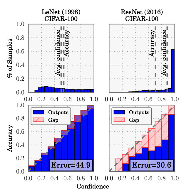
On Calibration of Modern Neural Networks
- Assumption: “the probability associated with the predicted class label should reflect its ground truth correctness likelihood.”
- Reality: “modern (large) neural networks are no longer well-calibrated”
- Solution: apply temperature scaling (extension of Platt scaling) on model outputs
Recent work on confident learning (cleanlab) focuses on identifying noisy labels (with calibration), which can then be properly relabeled and used for training.
1 2 | |
1 2 3 | |
Not all of these are necessarily labeling errors but situations where the predicted probabilities were not so confident. Therefore, it will be useful to attach the predicted outcomes along side results. This way, we can know if we need to relabel, upsample, etc. as mitigation strategies to improve our performance.
The operations in this section can be applied to entire labeled dataset to discover labeling errors via confidence learning.
Slicing
Just inspecting the overall and class metrics isn't enough to deploy our new version to production. There may be key slices of our dataset that we need to do really well on:
- Target / predicted classes (+ combinations)
- Features (explicit and implicit)
- Metadata (timestamps, sources, etc.)
- Priority slices / experience (minority groups, large users, etc.)
An easy way to create and evaluate slices is to define slicing functions.
1 2 3 | |
1 2 3 4 5 6 7 | |
1 2 3 4 | |
Here we're using Snorkel's slicing_function to create our different slices. We can visualize our slices by applying this slicing function to a relevant DataFrame using slice_dataframe.
1 2 | |
1 2 | |
We can define even more slicing functions and create a slices record array using the PandasSFApplier. The slices array has N (# of data points) items and each item has S (# of slicing functions) items, indicating whether that data point is part of that slice. Think of this record array as a masking layer for each slicing function on our data.
1 2 3 4 5 | |
rec.array([(0, 0), (0, 0), (0, 0), (0, 0), (0, 0), (0, 0), (0, 0), (0, 0),
           (1, 0) (0, 0) (0, 1) (0, 0) (0, 0) (1, 0) (0, 0) (0, 0) (0, 1) (0, 0)
           ...
           (0, 0), (0, 0), (0, 0), (0, 0), (0, 0), (0, 0), (0, 0), (0, 1),
           (0, 0), (0, 0)],
    dtype=[('nlp_cnn', '<i8'), ('short_text', '<i8')])
To calculate metrics for our slices, we could use snorkel.analysis.Scorer but we've implemented a version that will work for multiclass or multilabel scenarios.
1 2 3 4 5 6 7 8 9 10 11 12 13 | |
1 | |
{
  "nlp_llm": {
    "precision": 0.9642857142857143,
    "recall": 0.9642857142857143,
    "f1": 0.9642857142857143,
    "num_samples": 28
  },
  "short_text": {
    "precision": 1.0,
    "recall": 1.0,
    "f1": 1.0,
    "num_samples": 7
  }
}
Slicing can help identify sources of bias in our data. For example, our model has most likely learned to associated algorithms with certain applications such as CNNs used for computer vision or transformers used for NLP projects. However, these algorithms are not being applied beyond their initial use cases. We’d need ensure that our model learns to focus on the application over algorithm. This could be learned with:
- enough data (new or oversampling incorrect predictions)
- masking the algorithm (using text matching heuristics)
Interpretability
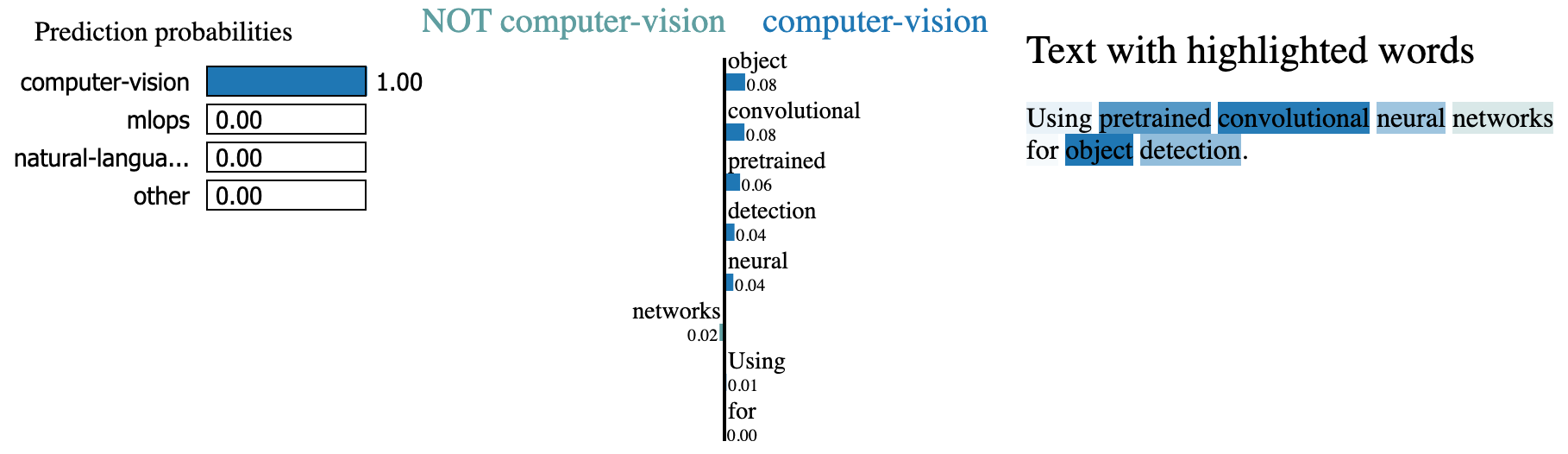
Besides just comparing predicted outputs with ground truth values, we can also inspect the inputs to our models. What aspects of the input are more influential towards the prediction? If the focus is not on the relevant features of our input, then we need to explore if there is a hidden pattern we're missing or if our model has learned to overfit on the incorrect features. We can use techniques such as SHAP (SHapley Additive exPlanations) or LIME (Local Interpretable Model-agnostic Explanations) to inspect feature importance. On a high level, these techniques learn which features have the most signal by assessing the performance in their absence. These inspections can be performed on a global level (ex. per-class) or on a local level (ex. single prediction).
1 2 | |
LimeTextExplainer.explain_instance function requires a classifier_fn that takes in a list of strings and outputs the predicted probabilities.
1 2 3 4 5 | |
1 2 3 4 | |
We can also use model-specific approaches to interpretability we we did in our embeddings lesson to identify the most influential n-grams in our text.
Behavioral testing
Besides just looking at metrics, we also want to conduct some behavioral sanity tests. Behavioral testing is the process of testing input data and expected outputs while treating the model as a black box. They don't necessarily have to be adversarial in nature but more along the types of perturbations we'll see in the real world once our model is deployed. A landmark paper on this topic is Beyond Accuracy: Behavioral Testing of NLP Models with CheckList which breaks down behavioral testing into three types of tests:
invariance: Changes should not affect outputs.1 2 3 4
# INVariance via verb injection (changes should not affect outputs) tokens = ["revolutionized", "disrupted"] texts = [f"Transformers applied to NLP have {token} the ML field." for token in tokens] [preprocessor.index_to_class[y_prob.argmax()] for y_prob in classifier_fn(texts=texts)]
['natural-language-processing', 'natural-language-processing']
directional: Change should affect outputs.1 2 3 4
# DIRectional expectations (changes with known outputs) tokens = ["text classification", "image classification"] texts = [f"ML applied to {token}." for token in tokens] [preprocessor.index_to_class[y_prob.argmax()] for y_prob in classifier_fn(texts=texts)]
['natural-language-processing', 'computer-vision']
minimum functionality: Simple combination of inputs and expected outputs.1 2 3 4
# Minimum Functionality Tests (simple input/output pairs) tokens = ["natural language processing", "mlops"] texts = [f"{token} is the next big wave in machine learning." for token in tokens] [preprocessor.index_to_class[y_prob.argmax()] for y_prob in classifier_fn(texts=texts)]
['natural-language-processing', 'mlops']
We'll learn how to systematically create tests in our testing lesson.
Online evaluation
Once we've evaluated our model's ability to perform on a static dataset we can run several types of online evaluation techniques to determine performance on actual production data. It can be performed using labels or, in the event we don't readily have labels, proxy signals.
- manually label a subset of incoming data to evaluate periodically.
- asking the initial set of users viewing a newly categorized content if it's correctly classified.
- allow users to report misclassified content by our model.
And there are many different experimentation strategies we can use to measure real-time performance before committing to replace our existing version of the system.
AB tests
AB testing involves sending production traffic to our current system (control group) and the new version (treatment group) and measuring if there is a statistical difference between the values for two metrics. There are several common issues with AB testing such as accounting for different sources of bias, such as the novelty effect of showing some users the new system. We also need to ensure that the same users continue to interact with the same systems so we can compare the results without contamination.
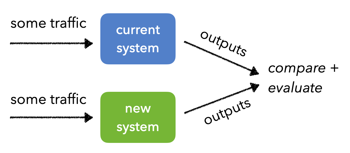
In many cases, if we're simply trying to compare the different versions for a certain metric, AB testing can take while before we reach statical significance since traffic is evenly split between the different groups. In this scenario, multi-armed bandits will be a better approach since they continuously assign traffic to the better performing version.
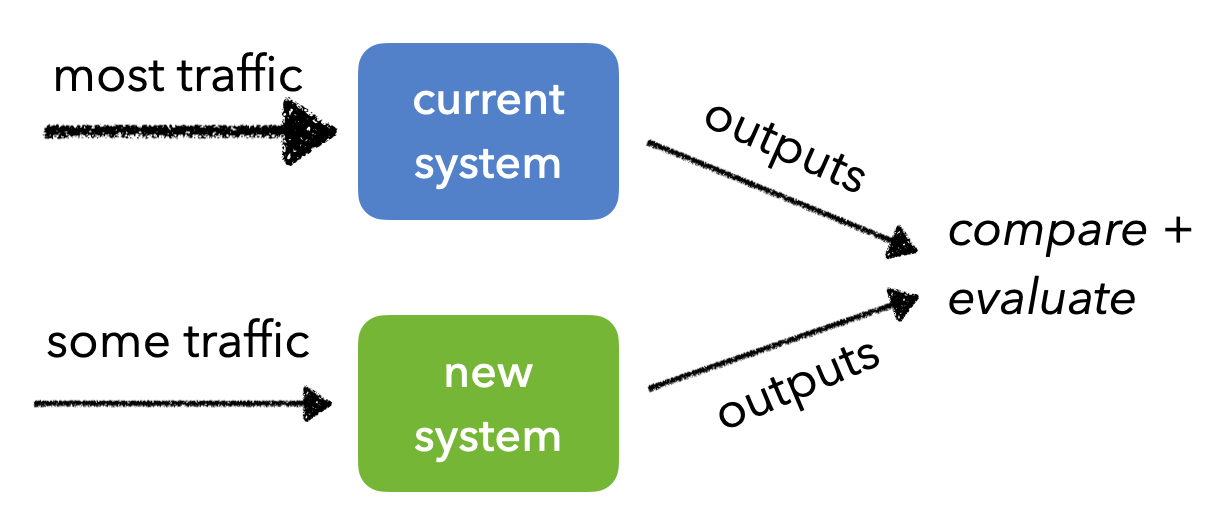
Canary tests
Canary tests involve sending most of the production traffic to the currently deployed system but sending traffic from a small cohort of users to the new system we're trying to evaluate. Again we need to make sure that the same users continue to interact with the same system as we gradually roll out the new system.
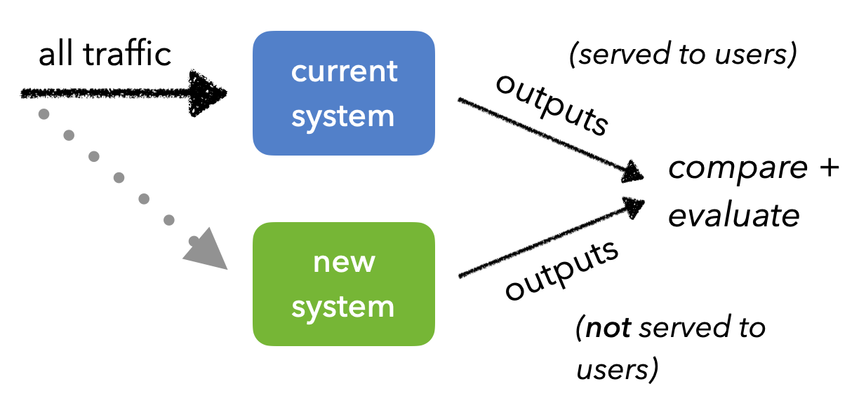
Shadow tests
Shadow testing involves sending the same production traffic to the different systems. We don't have to worry about system contamination and it's very safe compared to the previous approaches since the new system's results are not served. However, we do need to ensure that we're replicating as much of the production system as possible so we can catch issues that are unique to production early on. But overall, shadow testing is easy to monitor, validate operational consistency, etc.
What can go wrong?
If shadow tests allow us to test our updated system without having to actually serve the new results, why doesn't everyone adopt it?
Show answer
With shadow deployment, we'll miss out on any live feedback signals (explicit/implicit) from our users since users are not directly interacting with the product using our new version.
We also need to ensure that we're replicating as much of the production system as possible so we can catch issues that are unique to production early on. This is rarely possible because, while your ML system may be a standalone microservice, it ultimately interacts with an intricate production environment that has many dependencies.
Capability vs. alignment
We've seen the many different metrics that we'll want to calculate when it comes to evaluating our model but not all metrics mean the same thing. And this becomes very important when it comes to choosing the "best" model(s).
- capability: the ability of our model to perform a task, measured by the objective function we optimize for (ex. log loss)
- alignment: desired behavior of our model, measure by metrics that are not differentiable or don't account for misclassifications and probability differences (ex. accuracy, precision, recall, etc.)
While capability (ex. loss) and alignment (ex. accuracy) metrics may seem to be aligned, their differences can indicate issues in our data:
- ↓ accuracy, ↑ loss = large errors on lots of data (worst case)
- ↓ accuracy, ↓ loss = small errors on lots of data, distributions are close but tipped towards misclassifications (misaligned)
- ↑ accuracy, ↑ loss = large errors on some data (incorrect predictions have very skewed distributions)
- ↑ accuracy, ↓ loss = no/few errors on some data (best case)
Resources
- Model Evaluation, Model Selection, and Algorithm Selection in Machine Learning
- On Calibration of Modern Neural Networks
- Confident Learning: Estimating Uncertainty in Dataset Labels
- Automated Data Slicing for Model Validation
- SliceLine: Fast, Linear-Algebra-based Slice Finding for ML Model Debugging
- Distributionally Robust Neural Networks for Group Shifts
- No Subclass Left Behind: Fine-Grained Robustness in Coarse-Grained Classification Problems
- Model Patching: Closing the Subgroup Performance Gap with Data Augmentation
Upcoming live cohorts
Sign up for our upcoming live cohort, where we'll provide live lessons + QA, compute (GPUs) and community to learn everything in one day.
To cite this content, please use:
1 2 3 4 5 6 | |