📬 Receive new lessons straight to your inbox (once a month) and join 40K+
developers in learning how to responsibly deliver value with ML.
Overview
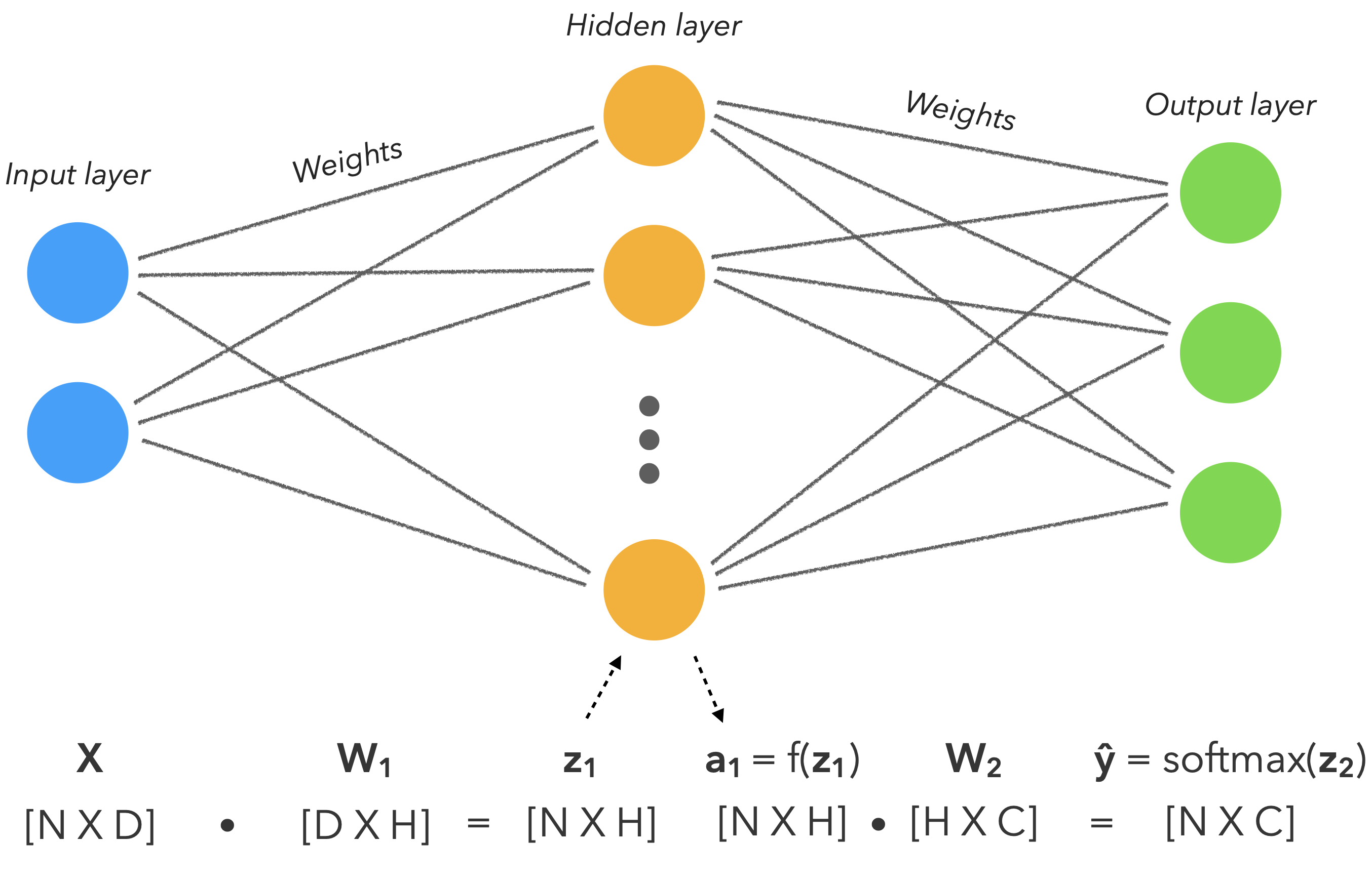
Our goal is to learn a model \(\hat{y}\) that models \(y\) given \(X\) . You'll notice that neural networks are just extensions of the generalized linear methods we've seen so far but with non-linear activation functions since our data will be highly non-linear.
\[ z_1 = XW_1 \]
\[ a_1 = f(z_1) \]
\[ z_2 = a_1W_2 \]
\[ \hat{y} = softmax(z_2) \]
Variable
Description
\(N\)
total numbers of samples
\(D\)
number of features
\(H\)
number of hidden units
\(C\)
number of classes
\(W_1\)
1st layer weights \(\in \mathbb{R}^{DXH}\)
\(z_1\)
outputs from first layer \(\in \mathbb{R}^{NXH}\)
\(f\)
non-linear activation function
\(a_1\)
activations from first layer \(\in \mathbb{R}^{NXH}\)
\(W_2\)
2nd layer weights \(\in \mathbb{R}^{HXC}\)
\(z_2\)
outputs from second layer \(\in \mathbb{R}^{NXC}\)
\(\hat{y}\)
prediction \(\in \mathbb{R}^{NXC}\)
(*) bias term (\(b\)) excluded to avoid crowding the notations
Objective:
Predict the probability of class \(y\) given the inputs \(X\). Non-linearity is introduced to model the complex, non-linear data.
Advantages:
Can model non-linear patterns in the data really well.
Disadvantages:
Overfits easily.
Computationally intensive as network increases in size.
Not easily interpretable.
Miscellaneous:
Future neural network architectures that we'll see use the MLP as a modular unit for feed forward operations (affine transformation (XW) followed by a non-linear operation).
Set up
We'll set our seeds for reproducibility.
12
importnumpyasnpimportrandom
1
SEED=1234
123
# Set seed for reproducibilitynp.random.seed(SEED)random.seed(SEED)
Load data
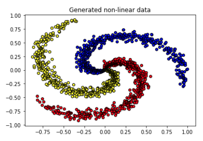
I created some non-linearly separable spiral data so let's go ahead and download it for our classification task.
deftrain_val_test_split(X,y,train_size):"""Split dataset into data splits."""X_train,X_,y_train,y_=train_test_split(X,y,train_size=TRAIN_SIZE,stratify=y)X_val,X_test,y_val,y_test=train_test_split(X_,y_,train_size=0.5,stratify=y_)returnX_train,X_val,X_test,y_train,y_val,y_test
In the previous lesson we wrote our own label encoder class to see the inner functions but this time we'll use scikit-learn LabelEncoder class which does the same operations as ours.
1
fromsklearn.preprocessingimportLabelEncoder
12
# Output vectorizerlabel_encoder=LabelEncoder()
1234
# Fit on train datalabel_encoder=label_encoder.fit(y_train)classes=list(label_encoder.classes_)print(f"classes: {classes}")
classes: ["c1", "c2", "c3"]
123456
# Convert labels to tokensprint(f"y_train[0]: {y_train[0]}")y_train=label_encoder.transform(y_train)y_val=label_encoder.transform(y_val)y_test=label_encoder.transform(y_test)print(f"y_train[0]: {y_train[0]}")
y_train[0]: c1
y_train[0]: 0
1234
# Class weightscounts=np.bincount(y_train)class_weights={i:1.0/countfori,countinenumerate(counts)}print(f"counts: {counts}\nweights: {class_weights}")
We need to standardize our data (zero mean and unit variance) so a specific feature's magnitude doesn't affect how the model learns its weights. We're only going to standardize the inputs X because our outputs y are class values.
1
fromsklearn.preprocessingimportStandardScaler
12
# Standardize the data (mean=0, std=1) using training dataX_scaler=StandardScaler().fit(X_train)
1234
# Apply scaler on training and test data (don't standardize outputs for classification)X_train=X_scaler.transform(X_train)X_val=X_scaler.transform(X_val)X_test=X_scaler.transform(X_test)
123
# Check (means should be ~0 and std should be ~1)print(f"X_test[0]: mean: {np.mean(X_test[:,0],axis=0):.1f}, std: {np.std(X_test[:,0],axis=0):.1f}")print(f"X_test[1]: mean: {np.mean(X_test[:,1],axis=0):.1f}, std: {np.std(X_test[:,1],axis=0):.1f}")
Before we get to our neural network, we're going to motivate non-linear activation functions by implementing a generalized linear model (logistic regression). We'll see why linear models (with linear activations) won't suffice for our dataset.
1
importtorch
12
# Set seed for reproducibilitytorch.manual_seed(SEED)
Model
We'll create our linear model using one layer of weights.
12
fromtorchimportnnimporttorch.nn.functionalasF
123
INPUT_DIM=X_train.shape[1]# X is 2-dimensionalHIDDEN_DIM=100NUM_CLASSES=len(classes)# 3 classes
1 2 3 4 5 6 7 8 910
classLinearModel(nn.Module):def__init__(self,input_dim,hidden_dim,num_classes):super(LinearModel,self).__init__()self.fc1=nn.Linear(input_dim,hidden_dim)self.fc2=nn.Linear(hidden_dim,num_classes)defforward(self,x_in):z=self.fc1(x_in)# linear activationz=self.fc2(z)returnz
# Convert data to tensorsX_train=torch.Tensor(X_train)y_train=torch.LongTensor(y_train)X_val=torch.Tensor(X_val)y_val=torch.LongTensor(y_val)X_test=torch.Tensor(X_test)y_test=torch.LongTensor(y_test)
1 2 3 4 5 6 7 8 9101112131415161718192021
# Trainingforepochinrange(NUM_EPOCHS):# Forward passy_pred=model(X_train)# Lossloss=loss_fn(y_pred,y_train)# Zero all gradientsoptimizer.zero_grad()# Backward passloss.backward()# Update weightsoptimizer.step()ifepoch%1==0:predictions=y_pred.max(dim=1)[1]# classaccuracy=accuracy_fn(y_pred=predictions,y_true=y_train)print(f"Epoch: {epoch} | loss: {loss:.2f}, accuracy: {accuracy:.1f}")
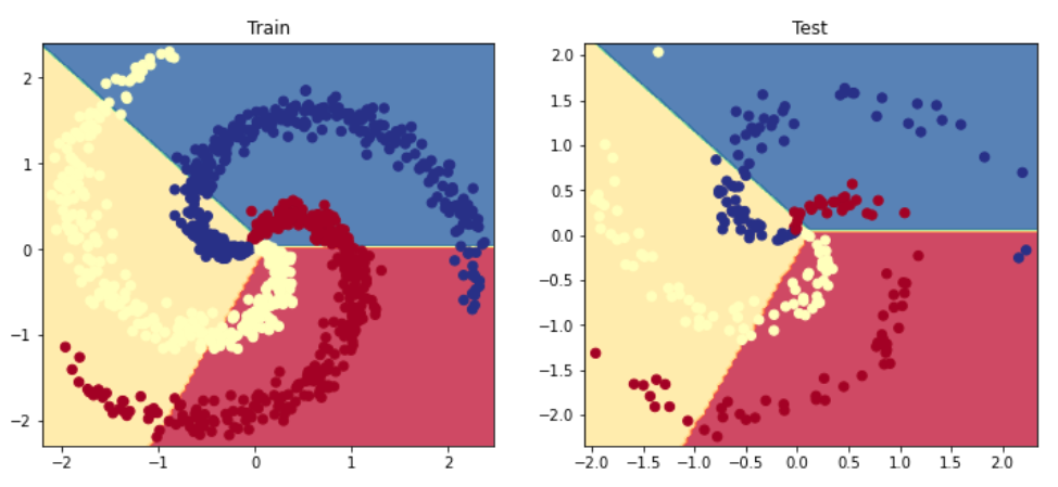
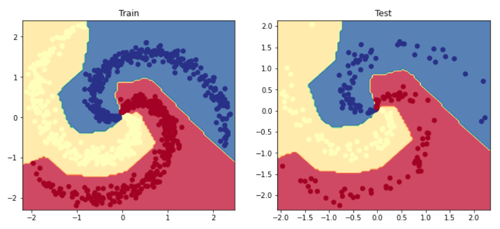
# Visualize the decision boundaryplt.figure(figsize=(12,5))plt.subplot(1,2,1)plt.title("Train")plot_multiclass_decision_boundary(model=model,X=X_train,y=y_train)plt.subplot(1,2,2)plt.title("Test")plot_multiclass_decision_boundary(model=model,X=X_test,y=y_test)plt.show()
Activation functions
Using the generalized linear method (logistic regression) yielded poor results because of the non-linearity present in our data yet our activation functions were linear. We need to use an activation function that can allow our model to learn and map the non-linearity in our data. There are many different options so let's explore a few.
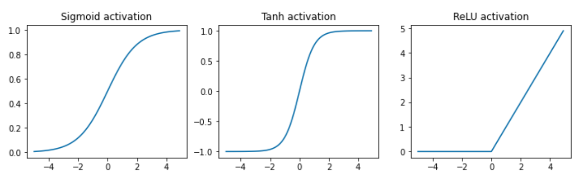
# Fig sizeplt.figure(figsize=(12,3))# Datax=torch.arange(-5.,5.,0.1)# Sigmoid activation (constrain a value between 0 and 1.)plt.subplot(1,3,1)plt.title("Sigmoid activation")y=torch.sigmoid(x)plt.plot(x.numpy(),y.numpy())# Tanh activation (constrain a value between -1 and 1.)plt.subplot(1,3,2)y=torch.tanh(x)plt.title("Tanh activation")plt.plot(x.numpy(),y.numpy())# Relu (clip the negative values to 0)plt.subplot(1,3,3)y=F.relu(x)plt.title("ReLU activation")plt.plot(x.numpy(),y.numpy())# Show plotsplt.show()
The ReLU activation function (\(max(0,z)\)) is by far the most widely used activation function for neural networks. But as you can see, each activation function has its own constraints so there are circumstances where you'll want to use different ones. For example, if we need to constrain our outputs between 0 and 1, then the sigmoid activation is the best choice.
In some cases, using a ReLU activation function may not be sufficient. For instance, when the outputs from our neurons are mostly negative, the activation function will produce zeros. This effectively creates a "dying ReLU" and a recovery is unlikely. To mitigate this effect, we could lower the learning rate or use alternative ReLU activations, ex. leaky ReLU or parametric ReLU (PReLU), which have a small slope for negative neuron outputs.
NumPy
Now let's create our multilayer perceptron (MLP) which is going to be exactly like the logistic regression model but with the activation function to map the non-linearity in our data.
It's normal to find the math and code in this section slightly complex. You can still read each of the steps to build intuition for when we implement this using PyTorch.
Our goal is to learn a model \(\hat{y}\) that models \(y\) given \(X\). You'll notice that neural networks are just extensions of the generalized linear methods we've seen so far but with non-linear activation functions since our data will be highly non-linear.
\[ z_1 = XW_1 \]
\[ a_1 = f(z_1) \]
\[ z_2 = a_1W_2 \]
\[ \hat{y} = softmax(z_2) \]
Initialize weights
Step 1: Randomly initialize the model's weights \(W\) (we'll cover more effective initialization strategies later in this lesson).
12345
# Initialize first layer's weightsW1=0.01*np.random.randn(INPUT_DIM,HIDDEN_DIM)b1=np.zeros((1,HIDDEN_DIM))print(f"W1: {W1.shape}")print(f"b1: {b1.shape}")
W1: (2, 100)
b1: (1, 100)
Model
Step 2: Feed inputs \(X\) into the model to do the forward pass and receive the probabilities.
First we pass the inputs into the first layer.
We'll apply the softmax function to normalize the logits and obtain class probabilities.
\[ \hat{y} = softmax(z_2) \]
12345
# Normalization via softmax to obtain class probabilitiesexp_logits=np.exp(logits)y_hat=exp_logits/np.sum(exp_logits,axis=1,keepdims=True)print(f"y_hat: {y_hat.shape}")print(f"sample: {y_hat[0]}")
Step 3: Compare the predictions \(\hat{y}\) (ex. [0.3, 0.3, 0.4]) with the actual target values \(y\) (ex. class 2 would look like [0, 0, 1]) with the objective (cost) function to determine loss \(J\). A common objective function for classification tasks is cross-entropy loss.
Step 5: Update the weights \(W\) using a small learning rate \(\alpha\). The updates will penalize the probability for the incorrect classes (\(j\)) and encourage a higher probability for the correct class (\(y\)).
defplot_multiclass_decision_boundary_numpy(model,X,y,savefig_fp=None):"""Plot the multiclass decision boundary for a model that accepts 2D inputs. Credit: https://cs231n.github.io/neural-networks-case-study/ Arguments: model {function} -- trained model with function model.predict(x_in). X {numpy.ndarray} -- 2D inputs with shape (N, 2). y {numpy.ndarray} -- 1D outputs with shape (N,). """# Axis boundariesx_min,x_max=X[:,0].min()-0.1,X[:,0].max()+0.1y_min,y_max=X[:,1].min()-0.1,X[:,1].max()+0.1xx,yy=np.meshgrid(np.linspace(x_min,x_max,101),np.linspace(y_min,y_max,101))# Create predictionsx_in=np.c_[xx.ravel(),yy.ravel()]y_pred=model.predict(x_in)y_pred=np.argmax(y_pred,axis=1).reshape(xx.shape)# Plot decision boundaryplt.contourf(xx,yy,y_pred,cmap=plt.cm.Spectral,alpha=0.8)plt.scatter(X[:,0],X[:,1],c=y,s=40,cmap=plt.cm.RdYlBu)plt.xlim(xx.min(),xx.max())plt.ylim(yy.min(),yy.max())# Plotifsavefig_fp:plt.savefig(savefig_fp,format="png")
123456789
# Visualize the decision boundaryplt.figure(figsize=(12,5))plt.subplot(1,2,1)plt.title("Train")plot_multiclass_decision_boundary_numpy(model=model,X=X_train,y=y_train)plt.subplot(1,2,2)plt.title("Test")plot_multiclass_decision_boundary_numpy(model=model,X=X_test,y=y_test)plt.show()
PyTorch
Now let's implement the same MLP in PyTorch.
Model
We'll be using two linear layers along with PyTorch Functional API's ReLU operation.
1 2 3 4 5 6 7 8 910
classMLP(nn.Module):def__init__(self,input_dim,hidden_dim,num_classes):super(MLP,self).__init__()self.fc1=nn.Linear(input_dim,hidden_dim)self.fc2=nn.Linear(hidden_dim,num_classes)defforward(self,x_in):z=F.relu(self.fc1(x_in))# ReLU activation function added!z=self.fc2(z)returnz
# Convert data to tensorsX_train=torch.Tensor(X_train)y_train=torch.LongTensor(y_train)X_val=torch.Tensor(X_val)y_val=torch.LongTensor(y_val)X_test=torch.Tensor(X_test)y_test=torch.LongTensor(y_test)
1 2 3 4 5 6 7 8 9101112131415161718192021
# Trainingforepochinrange(NUM_EPOCHS*10):# Forward passy_pred=model(X_train)# Lossloss=loss_fn(y_pred,y_train)# Zero all gradientsoptimizer.zero_grad()# Backward passloss.backward()# Update weightsoptimizer.step()ifepoch%10==0:predictions=y_pred.max(dim=1)[1]# classaccuracy=accuracy_fn(y_pred=predictions,y_true=y_train)print(f"Epoch: {epoch} | loss: {loss:.2f}, accuracy: {accuracy:.1f}")
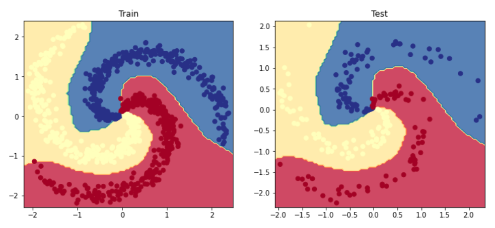
# Visualize the decision boundaryplt.figure(figsize=(12,5))plt.subplot(1,2,1)plt.title("Train")plot_multiclass_decision_boundary(model=model,X=X_train,y=y_train)plt.subplot(1,2,2)plt.title("Test")plot_multiclass_decision_boundary(model=model,X=X_test,y=y_test)plt.show()
Inference
Let's look at the inference operations when using our trained model.
12
# Inputs for inferenceX_infer=pd.DataFrame([{"X1":0.1,"X2":0.1}])
# Predicty_infer=F.softmax(model(torch.Tensor(X_infer)),dim=1)prob,_class=y_infer.max(dim=1)label=label_encoder.inverse_transform(_class.detach().numpy())[0]print(f"The probability that you have {label} is {prob.detach().numpy()[0]*100.0:.0f}%")
The probability that you have c1 is 92%
Initializing weights
So far we have been initializing weights with small random values but this isn't optimal for convergence during training. The objective is to initialize the appropriate weights such that our activations (outputs of layers) don't vanish (too small) or explode (too large), as either of these situations will hinder convergence. We can do this by sampling the weights uniformly from a bound distribution (many that take into account the precise activation function used) such that all activations have unit variance.
You may be wondering why we don't do this for every forward pass and that's a great question. We'll look at more advanced strategies that help with optimization like batch normalization, etc. in future lessons. Meanwhile you can check out other initializers here.
1
fromtorch.nnimportinit
1 2 3 4 5 6 7 8 910111213
classMLP(nn.Module):def__init__(self,input_dim,hidden_dim,num_classes):super(MLP,self).__init__()self.fc1=nn.Linear(input_dim,hidden_dim)self.fc2=nn.Linear(hidden_dim,num_classes)definit_weights(self):init.xavier_normal(self.fc1.weight,gain=init.calculate_gain("relu"))defforward(self,x_in):z=F.relu(self.fc1(x_in))# ReLU activation function added!z=self.fc2(z)returnz
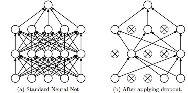
Dropout
A great technique to have our models generalize (perform well on test data) is to increase the size of your data but this isn't always an option. Fortunately, there are methods like regularization and dropout that can help create a more robust model.
Dropout is a technique (used only during training) that allows us to zero the outputs of neurons. We do this for dropout_p% of the total neurons in each layer and it changes every batch. Dropout prevents units from co-adapting too much to the data and acts as a sampling strategy since we drop a different set of neurons each time.
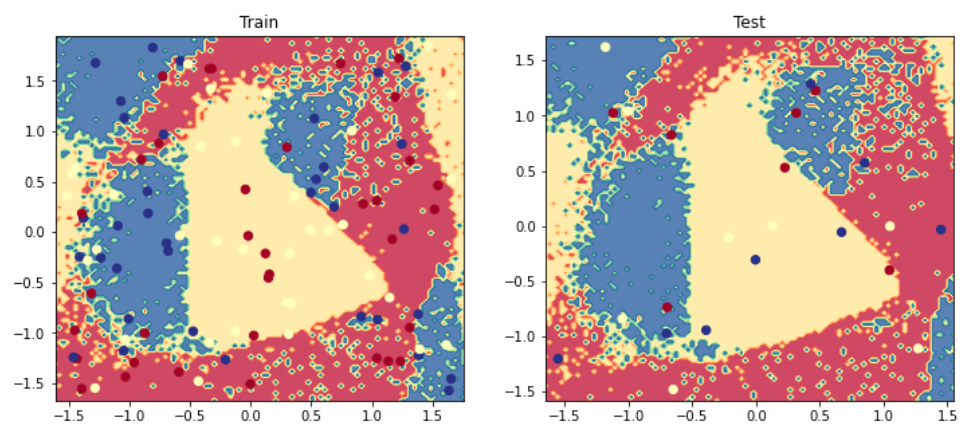
Though neural networks are great at capturing non-linear relationships they are highly susceptible to overfitting to the training data and failing to generalize on test data. Just take a look at the example below where we generate completely random data and are able to fit a model with \(2*N*C + D\) (where N = # of samples, C = # of classes and D = input dimension) hidden units. The training performance is good (~70%) but the overfitting leads to very poor test performance. We'll be covering strategies to tackle overfitting in future lessons.
1234
NUM_EPOCHS=500NUM_SAMPLES_PER_CLASS=50LEARNING_RATE=1e-1HIDDEN_DIM=2*NUM_SAMPLES_PER_CLASS*NUM_CLASSES+INPUT_DIM# 2*N*C + D
12345
# Generate random dataX=np.random.rand(NUM_SAMPLES_PER_CLASS*NUM_CLASSES,INPUT_DIM)y=np.array([[i]*NUM_SAMPLES_PER_CLASSforiinrange(NUM_CLASSES)]).reshape(-1)print("X: ",format(np.shape(X)))print("y: ",format(np.shape(y)))
# Standardize the inputs (mean=0, std=1) using training dataX_scaler=StandardScaler().fit(X_train)X_train=X_scaler.transform(X_train)X_val=X_scaler.transform(X_val)X_test=X_scaler.transform(X_test)
1234567
# Convert data to tensorsX_train=torch.Tensor(X_train)y_train=torch.LongTensor(y_train)X_val=torch.Tensor(X_val)y_val=torch.LongTensor(y_val)X_test=torch.Tensor(X_test)y_test=torch.LongTensor(y_test)
# Visualize the decision boundaryplt.figure(figsize=(12,5))plt.subplot(1,2,1)plt.title("Train")plot_multiclass_decision_boundary(model=model,X=X_train,y=y_train)plt.subplot(1,2,2)plt.title("Test")plot_multiclass_decision_boundary(model=model,X=X_test,y=y_test)plt.show()
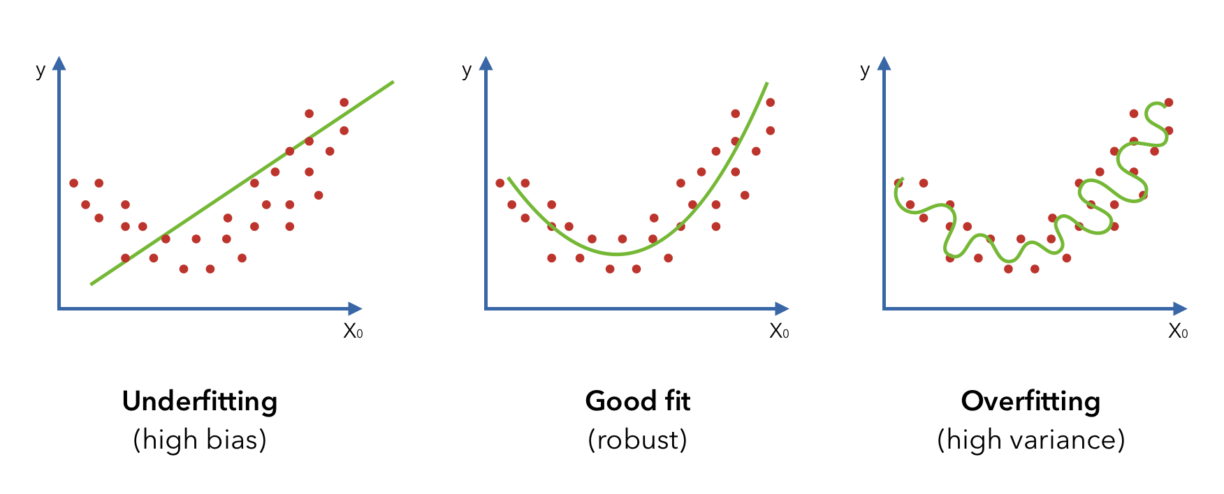
It's important that we experiment, starting with simple models that underfit (high bias) and improve it towards a good fit. Starting with simple models (linear/logistic regression) let's us catch errors without the added complexity of more sophisticated models (neural networks).
To cite this content, please use:
123456
@article{madewithml,author={Goku Mohandas},title={ Neural networks - Made With ML },howpublished={\url{https://madewithml.com/}},year={2023}}