Data Engineering for Machine Learning

View all lessons

Learn data engineering fundamentals by constructing a modern data stack for analytics and machine learning applications.

Goku Mohandas

· · ·

Repository · Notebook

Subscribe to our newsletter

📬 Receive new lessons straight to your inbox (once a month) and join 40K+ developers in learning how to responsibly deliver value with ML.

Intuition

So far we've had the convenience of using local CSV files as data source but in reality, our data can come from many disparate sources. Additionally, our processes around transforming and testing our data should ideally be moved upstream so that many different downstream processes can benefit from them. Our ML use case being just one among the many potential downstream applications. To address these shortcomings, we're going to learn about the fundamentals of data engineering and construct a modern data stack that can scale and provide high quality data for our applications.

View the data-engineering repository for all the code.

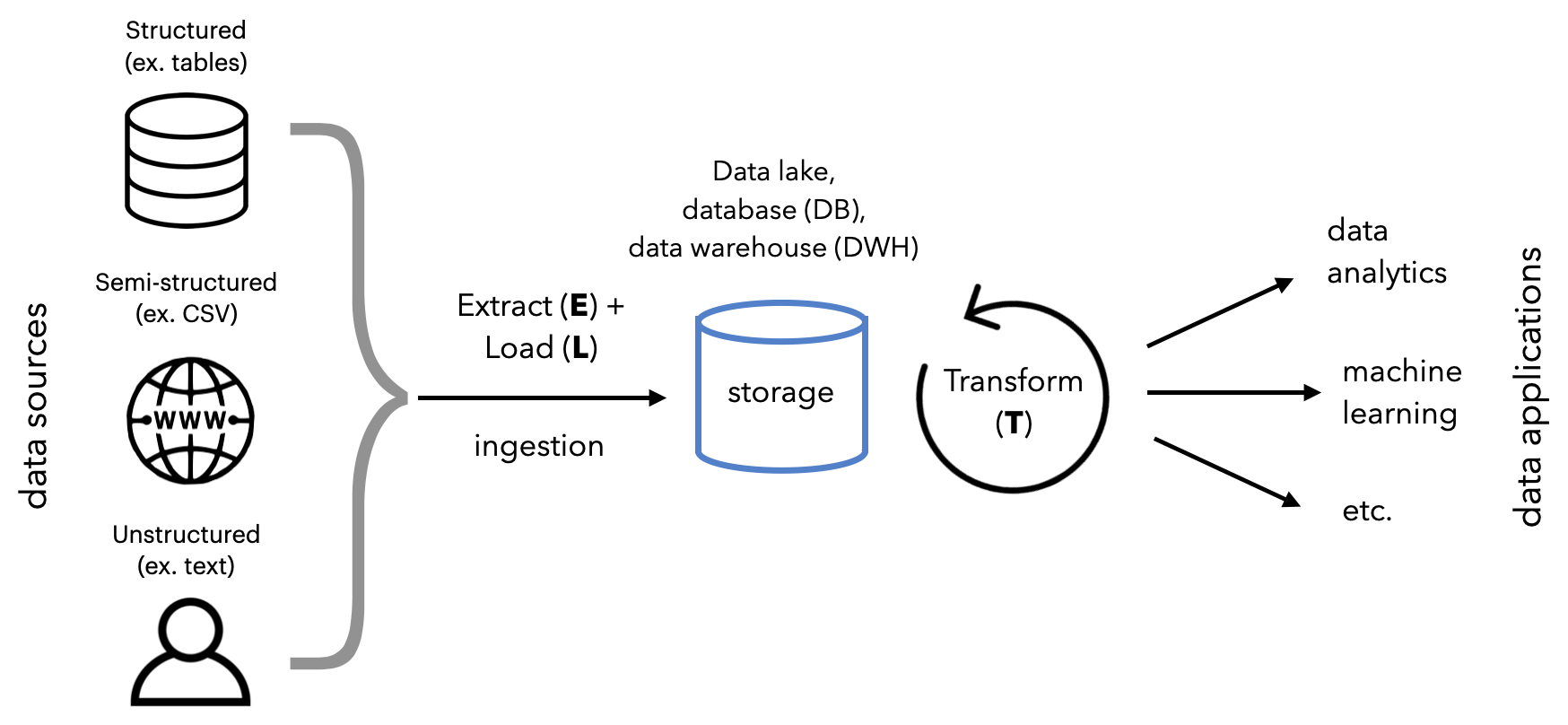
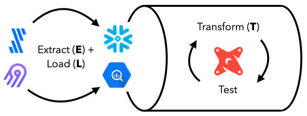
At a high level, we're going to:

Extract and Load data from sources to destinations.
Transform data for downstream applications.

This process is more commonly known as ELT, but there are variants such as ETL and reverse ETL, etc. They are all essentially the same underlying workflows but have slight differences in the order of data flow and where data is processed and stored.

Utility and simplicity

It can be enticing to set up a modern data stack in your organization, especially with all the hype. But it's very important to motivate utility and adding additional complexity:

Start with a use case that we already have data sources for and has direct impact on the business' bottom line (ex. user churn).
Start with the simplest infrastructure (source → database → report) and add complexity (in infrastructure, performance and team) as needed.

Data systems

Before we start working with our data, it's important to understand the different types of systems that our data can live in. So far in this course we've worked with files, but there are several types of data systems that are widely adopted in industry for different purposes.

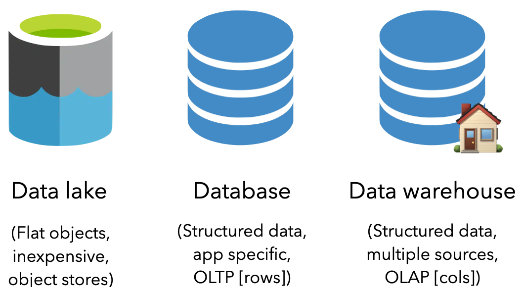
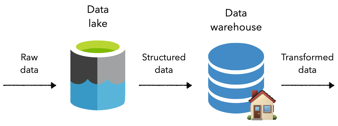
Data lake

A data lake is a flat data management system that stores raw objects. It's a great option for inexpensive storage and has the capability to hold all types of data (unstructured, semi-structured and structured). Object stores are becoming the standard for data lakes with default options across the popular cloud providers. Unfortunately, because data is stored as objects in a data lake, it's not designed for operating on structured data.

Popular data lake options include Amazon S3, Azure Blob Storage, Google Cloud Storage, etc.

Database

Another popular storage option is a database (DB), which is an organized collection of structured data that adheres to either:

relational schema (tables with rows and columns) often referred to as a Relational Database Management System (RDBMS) or SQL database.
non-relational (key/value, graph, etc.), often referred to as a non-relational database or NoSQL database.

A database is an online transaction processing (OLTP) system because it's typically used for day-to-day CRUD (create, read, update, delete) operations where typically information is accessed by rows. However, they're generally used to store data from one application and is not designed to hold data from across many sources for the purpose of analytics.

Popular database options include PostgreSQL, MySQL, MongoDB, Cassandra, etc.

Data warehouse

A data warehouse (DWH) is a type of database that's designed for storing structured data from many different sources for downstream analytics and data science. It's an online analytical processing (OLAP) system that's optimized for performing operations across aggregating column values rather than accessing specific rows.

Popular data warehouse options include SnowFlake, Google BigQuery, Amazon RedShift, Hive, etc.

Extract and load

The first step in our data pipeline is to extract data from a source and load it into the appropriate destination. While we could construct custom scripts to do this manually or on a schedule, an ecosystem of data ingestion tools have already standardized the entire process. They all come equipped with connectors that allow for extraction, normalization, cleaning and loading between sources and destinations. And these pipelines can be scaled, monitored, etc. all with very little to no code.

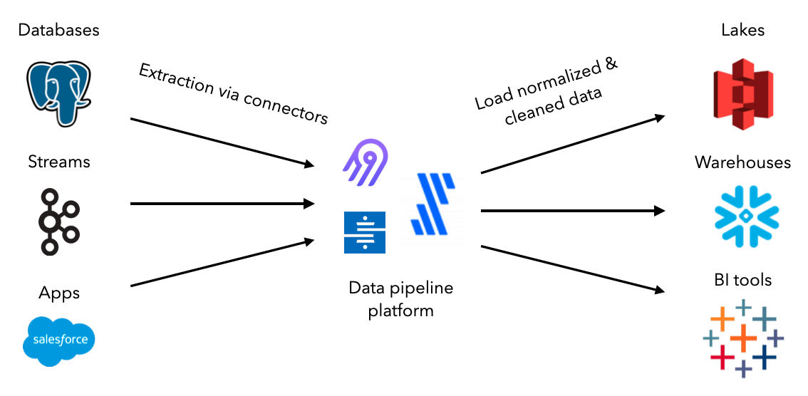
Popular data ingestion tools include Fivetran, Airbyte, Stitch, etc.

We're going to use the open-source tool Airbyte to create connections between our data sources and destinations. Let's set up Airbyte and define our data sources. As we progress in this lesson, we'll set up our destinations and create connections to extract and load data.

Ensure that we have Docker installed, but if not, download it here. For Windows users, be sure to have these configurations enabled.
In a parent directory, outside our project directory for the MLOps course, execute the following commands to load the Airbyte repository locally and launch the service.
```
git clone https://github.com/airbytehq/airbyte.git
cd airbyte
docker-compose up
```
After a few minutes, visit http://localhost:8000/ to view the launched Airbyte service.

Sources

Our data sources we want to extract from can be from anywhere. They could come from 3rd party apps, files, user click streams, physical devices, data lakes, databases, data warehouses, etc. But regardless of the source of our data, they type of data should fit into one of these categories:

structured: organized data stored in an explicit structure (ex. tables)
semi-structured: data with some structure but no formal schema or data types (web pages, CSV, JSON, etc.)
unstructured: qualitative data with no formal structure (text, images, audio, etc.)

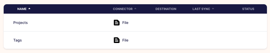
For our application, we'll define two data sources:

projects.csv: data containing projects with their ID, create date, title and description.
tags.csv: labels for each of project IDs in projects.csv

Ideally, these data assets would be retrieved from a database that contains projects that we extracted and perhaps another database that stores labels from our labeling team's workflows. However, for simplicity we'll use CSV files to demonstrate how to define a data source.

Define file source in Airbyte

We'll start our ELT process by defining the data source in Airbyte:

On our Airbyte UI, click on Sources on the left menu. Then click the + New source button on the top right corner.

Click on the Source type dropdown and choose File. This will open a view to define our file data source.

Name: Projects
URL: https://raw.githubusercontent.com/GokuMohandas/Made-With-ML/main/datasets/projects.csv
File Format: csv
Storage Provider: HTTPS: Public Web
Dataset Name: projects

Click the Set up source button and our data source will be tested and saved.

Repeat steps 1-3 for our tags data source as well:

Name: Tags
URL: https://raw.githubusercontent.com/GokuMohandas/Made-With-ML/main/datasets/tags.csv
File Format: csv
Storage Provider: HTTPS: Public Web
Dataset Name: tags

Destinations

Once we know the source we want to extract data from, we need to decide the destination to load it. The choice depends on what our downstream applications want to be able to do with the data. And it's also common to store data in one location (ex. data lake) and move it somewhere else (ex. data warehouse) for specific processing.

Set up Google BigQuery

Our destination will be a data warehouse since we'll want to use the data for downstream analytical and machine learning applications. We're going to use Google BigQuery which is free under Google Cloud's free tier for up to 10 GB storage and 1TB of queries (which is significantly more than we'll ever need for our purpose).

Log into your Google account and then head over to Google CLoud. If you haven't already used Google Cloud's free trial, you'll have to sign up. It's free and you won't be autocharged unless you manually upgrade your account. Once the trial ends, we'll still have the free tier which is more than plenty for us.
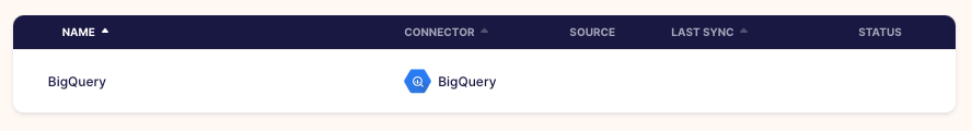
Go to the Google BigQuery page and click on the Go to console button.

We can create a new project by following these instructions which will lead us to the create project page.

Project name: made-with-ml  # Google will append a unique ID to the end of it
Location: No organization

Once the project has been created, refresh the page and we should see it (along with few other default projects from Google).

# Google BigQuery projects
├── made-with-ml-XXXXXX   👈 our project
├── bigquery-publicdata
├── imjasonh-storage
└── nyc-tlc

Console or code

Most cloud providers will allow us to do everything via console but also programmatically via API, Python, etc. For example, we manually create a project but we could've also done so with code as shown here.

Define BigQuery destination in Airbyte

Next, we need to establish the connection between Airbyte and BigQuery so that we can load the extracted data to the destination. In order to authenticate our access to BigQuery with Airbyte, we'll need to create a service account and generate a secret key. This is basically creating an identity with certain access that we can use for verification. Follow these instructions to create a service and generate the key file (JSON). Note down the location of this file because we'll be using it throughout this lesson. For example ours is /Users/goku/Downloads/made-with-ml-XXXXXX-XXXXXXXXXXXX.json.

On our Airbyte UI, click on Destinations on the left menu. Then click the + New destination button on the top right corner.

Click on the Destination type dropdown and choose BigQuery. This will open a view to define our file data source.

Name: BigQuery
Default Dataset ID: mlops_course  # where our data will go inside our BigQuery project
Project ID: made-with-ml-XXXXXX  # REPLACE this with your Google BiqQuery Project ID
Credentials JSON: SERVICE-ACCOUNT-KEY.json  # REPLACE this with your service account JSON location
Dataset location: US  # select US or EU, all other options will not be compatible with dbt later

Click the Set up destination button and our data destination will be tested and saved.

Connections

So we've set up our data sources (public CSV files) and destination (Google BigQuery data warehouse) but they haven't been connected yet. To create the connection, we need to think about a few aspects.

Frequency

How often do we want to extract data from the sources and load it into the destination?

batch: extracting data in batches, usually following a schedule (ex. daily) or when an event of interest occurs (ex. new data count)
streaming: extracting data in a continuous stream (using tools like Kafka, Kinesis, etc.)

Micro-batch

As we keep decreasing the time between batch ingestion (ex. towards 0), do we have stream ingestion? Not exactly. Batch processing is deliberately deciding to extract data from a source at a given interval. As that interval becomes <15 minutes, it's referred to as a micro-batch (many data warehouses allow for batch ingestion every 5 minutes). However, with stream ingestion, the extraction process is continuously on and events will keep being ingested.

Start simple

In general, it's a good idea to start with batch ingestion for most applications and slowly add the complexity of streaming ingestion (and additional infrastructure). This was we can prove that downstream applications are finding value from the data source and evolving to streaming later should only improve things.

We'll learn more about the different system design implications of batch vs. stream in our systems design lesson.

Connecting File source to BigQuery destination

Now we're ready to create the connection between our sources and destination:

On our Airbyte UI, click on Connections on the left menu. Then click the + New connection button on the top right corner.
Under Select a existing source, click on the Source dropdown and choose Projects and click Use existing source.

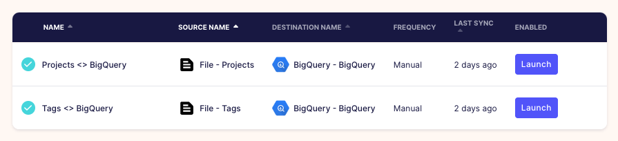
Under Select a existing destination, click on the Destination dropdown and choose BigQuery and click Use existing destination.

Connection name: Projects <> BigQuery
Replication frequency: Manual
Destination Namespace: Mirror source structure
Normalized tabular data: True  # leave this selected

Click the Set up connection button and our connection will be tested and saved.
Repeat the same for our Tags source with the same BigQuery destination.

Notice that our sync mode is Full refresh | Overwrite which means that every time we sync data from our source, it'll overwrite the existing data in our destination. As opposed to Full refresh | Append which will add entries from the source to bottom of the previous syncs.

Data sync

Our replication frequency is Manual because we'll trigger the data syncs ourselves:

On our Airbyte UI, click on Connections on the left menu. Then click the Projects <> BigQuery connection we set up earlier.
Press the 🔄 Sync now button and once it's completed we'll see that the projects are now in our BigQuery data warehouse.
Repeat the same with our Tags <> BigQuery connection.

# Inside our data warehouse
made-with-ml-XXXXXX               - Project
└── mlops_course                  - Dataset
│   ├── _airbyte_raw_projects     - table
│   ├── _airbyte_raw_tags         - table
│   ├── projects                  - table
│   └── tags                      - table

In our orchestration lesson, we'll use Airflow to programmatically execute the data sync.

We can easily explore and query this data using SQL directly inside our warehouse:

On our BigQuery project page, click on the 🔍 QUERY button and select In new tab.

Run the following SQL statement and view the data:

SELECT *
FROM `made-with-ml-XXXXXX.mlops_course.projects`
LIMIT 1000



  
    
      
      id
      created_on
      title
      description
    
  
  
    
      0
      6
      2020-02-20 06:43:18
      Comparison between YOLO and RCNN on real world...
      Bringing theory to experiment is cool. We can ...
    
    
      1
      7
      2020-02-20 06:47:21
      Show, Infer & Tell: Contextual Inference for C...
      The beauty of the work lies in the way it arch...
    
    
      2
      9
      2020-02-24 16:24:45
      Awesome Graph Classification
      A collection of important graph embedding, cla...
    
    
      3
      15
      2020-02-28 23:55:26
      Awesome Monte Carlo Tree Search
      A curated list of Monte Carlo tree search papers...
    
    
      4
      19
      2020-03-03 13:54:31
      Diffusion to Vector
      Reference implementation of Diffusion2Vec (Com...

Best practices

With the advent of cheap storage and cloud SaaS options to manage them, it's become a best practice to store raw data into data lakes. This allows for storage of raw, potentially unstructured, data without having to justify storage with downstream applications. When we do need to transform and process the data, we can move it to a data warehouse so can perform those operations efficiently.

Transform

Once we've extracted and loaded our data, we need to transform the data so that it's ready for downstream applications. These transformations are different from the preprocessing we've seen before but are instead reflective of business logic that's agnostic to downstream applications. Common transformations include defining schemas, filtering, cleaning and joining data across tables, etc. While we could do all of these things with SQL in our data warehouse (save queries as tables or views), dbt delivers production functionality around version control, testing, documentation, packaging, etc. out of the box. This becomes crucial for maintaining observability and high quality data workflows.

Popular transformation tools include dbt, Matillion, custom jinja templated SQL, etc.

Note

In addition to data transformations, we can also process the data using large-scale analytics engines like Spark, Flink, etc.

dbt Cloud

Now we're ready to transform our data in our data warehouse using dbt. We'll be using a developer account on dbt Cloud (free), which provides us with an IDE, unlimited runs, etc.

We'll learn how to use the dbt-core in our orchestration lesson. Unlike dbt Cloud, dbt core is completely open-source and we can programmatically connect to our data warehouse and perform transformations.

Create a free account and verify it.
Go to https://cloud.getdbt.com/ to get set up.
Click continue and choose BigQuery as the database.
Click Upload a Service Account JSON file and upload our file to autopopulate everything.
Click the Test > Continue.
Click Managed repository and name it dbt-transforms (or anything else you want).
Click Create > Continue > Skip and complete.
This will open the project page and click >_ Start Developing button.
This will open the IDE where we can click 🗂 initialize your project.

Now we're ready to start developing our models:

Click the ··· next to the models directory on the left menu.
Click New folder called models/labeled_projects.
Create a New file under models/labeled_projects called labeled_projects.sql.
Repeat for another file under models/labeled_projects called schema.yml.

dbt-cloud-XXXXX-dbt-transforms
├── ...
├── models
│   ├── example
│   └── labeled_projects
│   │   ├── labeled_projects.sql
│   │   └── schema.yml
├── ...
└── README.md

Joins

Inside our models/labeled_projects/labeled_projects.sql file we'll create a view that joins our project data with the appropriate tags. This will create the labeled data necessary for downstream applications such as machine learning models. Here we're joining based on the matching id between the projects and tags:

-- models/labeled_projects/labeled_projects.sql
SELECT p.id, created_on, title, description, tag
FROM `made-with-ml-XXXXXX.mlops_course.projects` p  -- REPLACE
LEFT JOIN `made-with-ml-XXXXXX.mlops_course.tags` t  -- REPLACE
ON p.id = t.id

We can view the queried results by clicking the Preview button and view the data lineage as well.

Schemas

Inside our models/labeled_projects/schema.yml file we'll define the schemas for each of the features in our transformed data. We also define several tests that each feature should pass. View the full list of dbt tests but note that we'll use Great Expectations for more comprehensive tests when we orchestrate all these data workflows in our orchestration lesson.

# models/labeled_projects/schema.yml

version: 2

models:
    - name: labeled_projects
      description: "Tags for all projects"
      columns:
          - name: id
            description: "Unique ID of the project."
            tests:
                - unique
                - not_null
          - name: title
            description: "Title of the project."
            tests:
                - not_null
          - name: description
            description: "Description of the project."
            tests:
                - not_null
          - name: tag
            description: "Labeled tag for the project."
            tests:
                - not_null

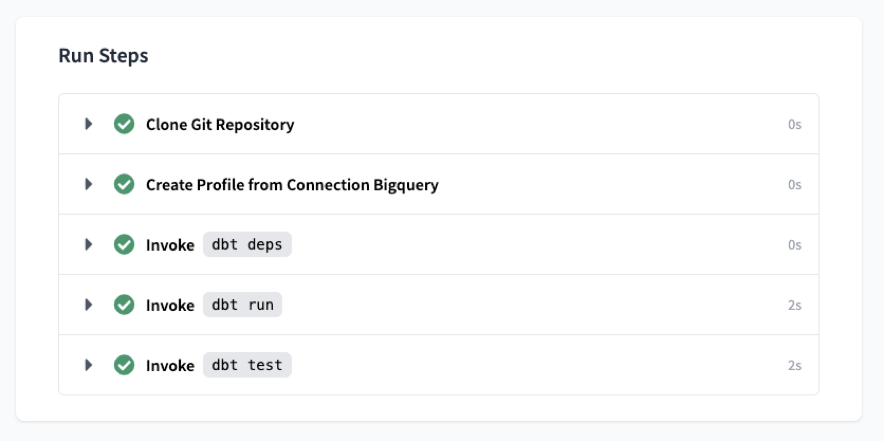
Runs

At the bottom of the IDE, we can execute runs based on the transformations we've defined. We'll run each of the following commands and once they finish, we can see the transformed data inside our data warehouse.

dbt run
dbt test

Once these commands run successfully, we're ready to move our transformations to a production environment where we can insert this view in our data warehouse.

Jobs

In order to apply these transformations to the data in our data warehouse, it's best practice to create an Environment and then define Jobs:

Click Environments on the left menu > New Environment button (top right corner) and fill out the details:
```
Name: Production
Type: Deployment
...
Dataset: mlops_course
```

Click New Job with the following details and then click Save (top right corner).

Name: Transform
Environment: Production
Commands: dbt run
          dbt test
Schedule: uncheck "RUN ON SCHEDULE"

Click Run Now and view the transformed data in our data warehouse under a view called labeled_projects.

# Inside our data warehouse
made-with-ml-XXXXXX               - Project
└── mlops_course                  - Dataset
│   ├── _airbyte_raw_projects     - table
│   ├── _airbyte_raw_tags         - table
│   ├── labeled_projects          - view
│   ├── projects                  - table
│   └── tags                      - table

There is so much more to dbt so be sure to check out their official documentation to really customize any workflows. And be sure to check out our orchestration lesson where we'll programmatically create and execute our dbt transformations.

Implementations

Hopefully we created our data stack for the purpose of gaining some actionable insight about our business, users, etc. Because it's these use cases that dictate which sources of data we extract from, how often and how that data is stored and transformed. Downstream applications of our data typically fall into one of these categories:

data analytics: use cases focused on reporting trends, aggregate views, etc. via charts, dashboards, etc.for the purpose of providing operational insight for business stakeholders.

🛠 Popular tools: Tableau, Looker, Metabase, Superset, etc.
machine learning: use cases centered around using the transformed data to construct predictive models (forecasting, personalization, etc.).

While it's very easy to extract data from our data warehouse:

pip install google-cloud-bigquery==1.21.0

from google.cloud import bigquery
from google.oauth2 import service_account

# Replace these with your own values
project_id = "made-with-ml-XXXXXX"  # REPLACE
SERVICE_ACCOUNT_KEY_JSON = "/Users/goku/Downloads/made-with-ml-XXXXXX-XXXXXXXXXXXX.json"  # REPLACE

# Establish connection
credentials = service_account.Credentials.from_service_account_file(SERVICE_ACCOUNT_KEY_JSON)
client = bigquery.Client(credentials= credentials, project=project_id)

# Query data
query_job = client.query("""
   SELECT *
   FROM mlops_course.labeled_projects""")
results = query_job.result()
results.to_dataframe().head()

	id	created_on	title	description	tag
0	1994.0	2020-07-29 04:51:30	Understanding the Effectivity of Ensembles in ...	The report explores the ideas presented in Dee...	computer-vision
1	1506.0	2020-06-19 06:26:17	Using GitHub Actions for MLOps & Data Science	A collection of resources on how to facilitate...	mlops
2	807.0	2020-05-11 02:25:51	Introduction to Machine Learning Problem Framing	This course helps you frame machine learning (...	mlops
3	1204.0	2020-06-05 22:56:38	Snaked: Classifying Snake Species using Images	Proof of concept that it is possible to identi...	computer-vision
4	1706.0	2020-07-04 11:05:28	PokeZoo	A deep learning based web-app developed using ...	computer-vision

Warning

Check out our notebook where we extract the transformed data from our data warehouse. We do this in a separate notebook because it requires the google-cloud-bigquery package and until dbt loosens it's Jinja versioning constraints... it'll have to be done in a separate environment. However, downstream applications are typically analytics or ML applications which have their own environments anyway so these conflicts are not inhibiting.

many of the analytics (ex. dashboards) and machine learning solutions (ex. feature stores) allow for easy connection to our data warehouses so that workflows can be triggered when an event occurs or on a schedule. We're going to take this a step further in the next lesson where we'll use a central orchestration platform to control all these workflows.

Analytics first, then ML

It's a good idea for the first several applications to be analytics and reporting based in order to establish a robust data stack. These use cases typically just involve displaying data aggregations and trends, as opposed to machine learning systems that involve additional complex infrastructure and workflows.

Observability

When we create complex data workflows like this, observability becomes a top priority. Data observability is the general concept of understanding the condition of data in our system and it involves:

data quality: testing and monitoring our data quality after every step (schemas, completeness, recency, etc.).
data lineage: mapping the where data comes from and how it's being transformed as it moves through our pipelines.
discoverability: enabling discovery of the different data sources and features for downstream applications.
privacy + security: are the different data assets treated and restricted appropriately amongst the applications?

Popular observability tools include Monte Carlo, Bigeye, etc.

Considerations

The data stack ecosystem to create the robust data workflows is growing and maturing. However, it can be overwhelming when it comes to choosing the best tooling options, especially as needs change over time. Here are a few important factors to consider when making a tooling decision in this space:

What is the cost per time per employee? Some of the tooling options can rack up quite the bill!
Does the tool have the proper connectors to integrate with our data sources and the rest of the stack?
Does the tool fit with our team's technical aptitude (SQL, Spark, Python, etc.)?
What kind of support does the tool offer (enterprise, community, etc.)?

Upcoming live cohorts

Sign up for our upcoming live cohort, where we'll provide live lessons + QA, compute (GPUs) and community to learn everything in one day.

To cite this content, please use:

@article{madewithml,
    author       = {Goku Mohandas},
    title        = { Data engineering - Made With ML },
    howpublished = {\url{https://madewithml.com/}},
    year         = {2023}
}

	id	created_on	title	description
0	6	2020-02-20 06:43:18	Comparison between YOLO and RCNN on real world...	Bringing theory to experiment is cool. We can ...
1	7	2020-02-20 06:47:21	Show, Infer & Tell: Contextual Inference for C...	The beauty of the work lies in the way it arch...
2	9	2020-02-24 16:24:45	Awesome Graph Classification	A collection of important graph embedding, cla...
3	15	2020-02-28 23:55:26	Awesome Monte Carlo Tree Search	A curated list of Monte Carlo tree search papers...
4	19	2020-03-03 13:54:31	Diffusion to Vector	Reference implementation of Diffusion2Vec (Com...