Monitoring Machine Learning Systems

Subscribe to our newsletter
📬 Receive new lessons straight to your inbox (once a month) and join 40K+ developers in learning how to responsibly deliver value with ML.
Intuition
Even though we've trained and thoroughly evaluated our model, the real work begins once we deploy to production. This is one of the fundamental differences between traditional software engineering and ML development. Traditionally, with rule based, deterministic, software, the majority of the work occurs at the initial stage and once deployed, our system works as we've defined it. But with machine learning, we haven't explicitly defined how something works but used data to architect a probabilistic solution. This approach is subject to natural performance degradation over time, as well as unintended behavior, since the data exposed to the model will be different from what it has been trained on. This isn't something we should be trying to avoid but rather understand and mitigate as much as possible. In this lesson, we'll understand the short comings from attempting to capture performance degradation in order to motivate the need for drift detection.
Tip
We highly recommend that you explore this lesson after completing the previous lessons since the topics (and code) are iteratively developed. We did, however, create the monitoring-ml repository for a quick overview with an interactive notebook.
System health
The first step to insure that our model is performing well is to ensure that the actual system is up and running as it should. This can include metrics specific to service requests such as latency, throughput, error rates, etc. as well as infrastructure utilization such as CPU/GPU utilization, memory, etc.
Fortunately, most cloud providers and even orchestration layers will provide this insight into our system's health for free through a dashboard. In the event we don't, we can easily use Grafana, Datadog, etc. to ingest system performance metrics from logs to create a customized dashboard and set alerts.
Performance
Unfortunately, just monitoring the system's health won't be enough to capture the underlying issues with our model. So, naturally, the next layer of metrics to monitor involves the model's performance. These could be quantitative evaluation metrics that we used during model evaluation (accuracy, precision, f1, etc.) but also key business metrics that the model influences (ROI, click rate, etc.).
It's usually never enough to just analyze the cumulative performance metrics across the entire span of time since the model has been deployed. Instead, we should also inspect performance across a period of time that's significant for our application (ex. daily). These sliding metrics might be more indicative of our system's health and we might be able to identify issues faster by not obscuring them with historical data.
👉 Follow along interactive notebook in the monitoring-ml repository as we implement the concepts below.
1 2 3 4 | |
1 2 3 4 5 | |
1 2 3 | |
Average cumulative f1 on the last day: 93.7
1 2 3 4 | |
Average sliding f1 on the last day: 88.6
1 2 3 4 5 | |
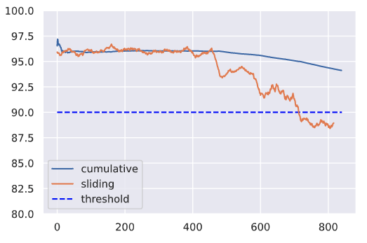
We may need to monitor metrics at various window sizes to catch performance degradation as soon as possible. Here we're monitoring the overall f1 but we can do the same for slices of data, individual classes, etc. For example, if we monitor the performance on a specific tag, we may be able to quickly catch new algorithms that were released for that tag (ex. new transformer architecture).
Delayed outcomes
We may not always have the ground-truth outcomes available to determine the model's performance on production inputs. This is especially true if there is significant lag or annotation is required on the real-world data. To mitigate this, we could:
- devise an approximate signal that can help us estimate the model's performance. For example, in our tag prediction task, we could use the actual tags that an author attributes to a project as the intermediary labels until we have verified labels from an annotation pipeline.
- label a small subset of our live dataset to estimate performance. This subset should try to be representative of the various distributions in the live data.
Importance weighting
However, approximate signals are not always available for every situation because there is no feedback on the ML system’s outputs or it’s too delayed. For these situations, a recent line of research relies on the only component that’s available in all situations: the input data.
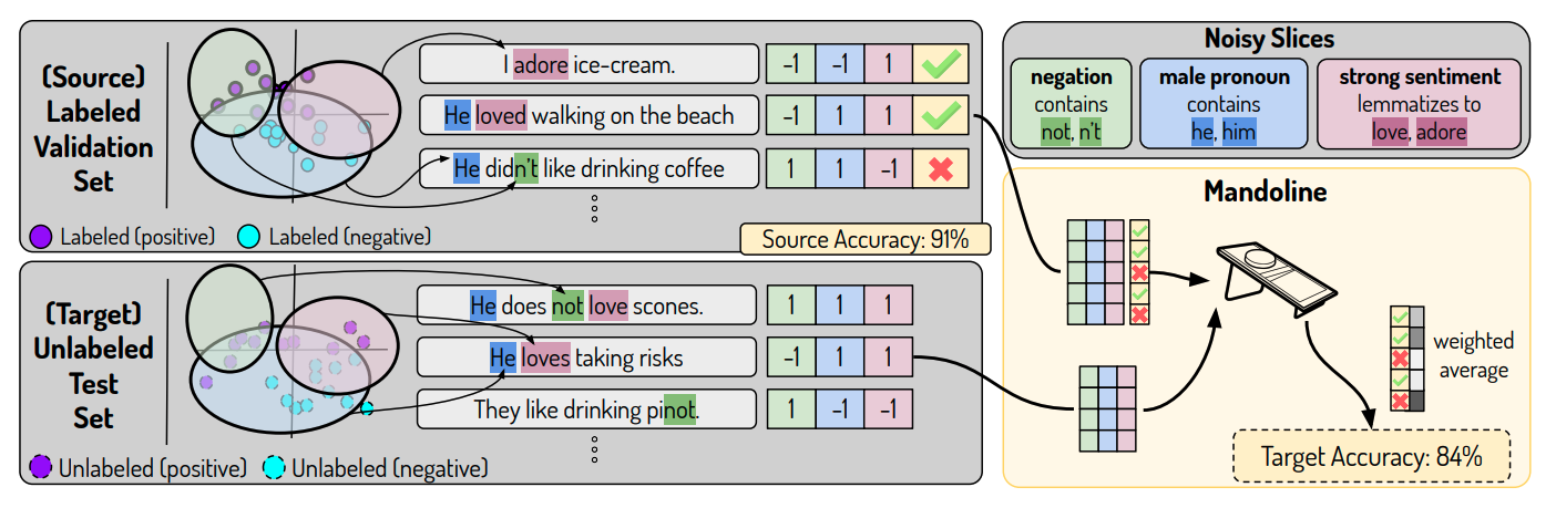
The core idea is to develop slicing functions that may potentially capture the ways our data may experience distribution shift. These slicing functions should capture obvious slices such as class labels or different categorical feature values but also slices based on implicit metadata (hidden aspects of the data that are not explicit feature columns). These slicing functions are then applied to our labeled dataset to create matrices with the corresponding labels. The same slicing functions are applied to our unlabeled production data to approximate what the weighted labels would be. With this, we can determine the approximate performance! The intuition here is that we can better approximate performance on our unlabeled dataset based on the similarity between the labeled slice matrix and unlabeled slice matrix. A core dependency of this assumption is that our slicing functions are comprehensive enough that they capture the causes of distributional shift.
Warning
If we wait to catch the model decay based on the performance, it may have already caused significant damage to downstream business pipelines that are dependent on it. We need to employ more fine-grained monitoring to identify the sources of model drift prior to actual performance degradation.
Drift
We need to first understand the different types of issues that can cause our model's performance to decay (model drift). The best way to do this is to look at all the moving pieces of what we're trying to model and how each one can experience drift.
| Entity | Description | Drift |
|---|---|---|
| \(X\) | inputs (features) | data drift \(\rightarrow P(X) \neq P_{ref}(X)\) |
| \(y\) | outputs (ground-truth) | target drift \(\rightarrow P(y) \neq P_{ref}(y)\) |
| \(P(y \vert X)\) | actual relationship between \(X\) and \(y\) | concept drift \(\rightarrow P(y \vert X) \neq P_{ref}(y \vert X)\) |
Data drift
Data drift, also known as feature drift or covariate shift, occurs when the distribution of the production data is different from the training data. The model is not equipped to deal with this drift in the feature space and so, it's predictions may not be reliable. The actual cause of drift can be attributed to natural changes in the real-world but also to systemic issues such as missing data, pipeline errors, schema changes, etc. It's important to inspect the drifted data and trace it back along it's pipeline to identify when and where the drift was introduced.
Warning
Besides just looking at the distribution of our input data, we also want to ensure that the workflows to retrieve and process our input data is the same during training and serving to avoid training-serving skew. However, we can skip this step if we retrieve our features from the same source location for both training and serving, ie. from a feature store.
As data starts to drift, we may not yet notice significant decay in our model's performance, especially if the model is able to interpolate well. However, this is a great opportunity to potentially retrain before the drift starts to impact performance.
Target drift
Besides just the input data changing, as with data drift, we can also experience drift in our outcomes. This can be a shift in the distributions but also the removal or addition of new classes with categorical tasks. Though retraining can mitigate the performance decay caused target drift, it can often be avoided with proper inter-pipeline communication about new classes, schema changes, etc.
Concept drift
Besides the input and output data drifting, we can have the actual relationship between them drift as well. This concept drift renders our model ineffective because the patterns it learned to map between the original inputs and outputs are no longer relevant. Concept drift can be something that occurs in various patterns:
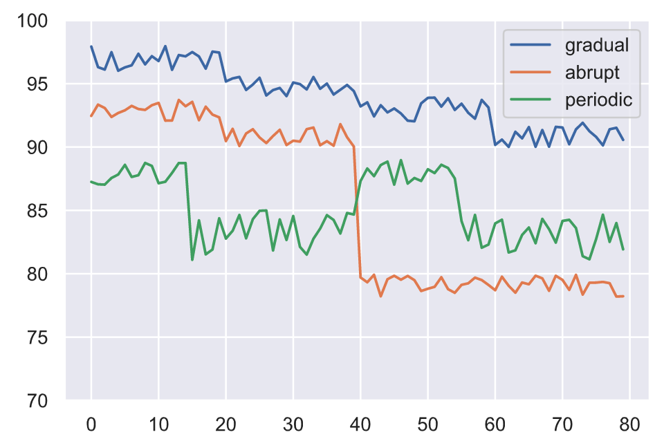
- gradually over a period of time
- abruptly as a result of an external event
- periodically as a result of recurring events
All the different types of drift we discussed can can occur simultaneously which can complicated identifying the sources of drift.
Locating drift
Now that we've identified the different types of drift, we need to learn how to locate and how often to measure it. Here are the constraints we need to consider:
- reference window: the set of points to compare production data distributions with to identify drift.
- test window: the set of points to compare with the reference window to determine if drift has occurred.
Since we're dealing with online drift detection (ie. detecting drift in live production data as opposed to past batch data), we can employ either a fixed or sliding window approach to identify our set of points for comparison. Typically, the reference window is a fixed, recent subset of the training data while the test window slides over time.
Scikit-multiflow provides a toolkit for concept drift detection techniques directly on streaming data. The package offers windowed, moving average functionality (including dynamic preprocessing) and even methods around concepts like gradual concept drift.
We can also compare across various window sizes simultaneously to ensure smaller cases of drift aren't averaged out by large window sizes.
Measuring drift
Once we have the window of points we wish to compare, we need to know how to compare them.
1 2 3 4 | |
1 2 3 4 5 6 7 | |
Expectations
The first form of measurement can be rule-based such as validating expectations around missing values, data types, value ranges, etc. as we did in our data testing lesson. The difference now is that we'll be validating these expectations on live production data.
1 2 | |
1 2 3 4 | |
1 2 | |
{'evaluated_expectations': 2,
 'success_percent': 100.0,
 'successful_expectations': 2,
 'unsuccessful_expectations': 0}
1 2 | |
{'evaluated_expectations': 2,
 'success_percent': 50.0,
 'successful_expectations': 1,
 'unsuccessful_expectations': 1}
Once we've validated our rule-based expectations, we need to quantitatively measure drift across the different features in our data.
Univariate
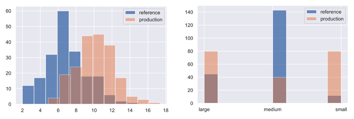
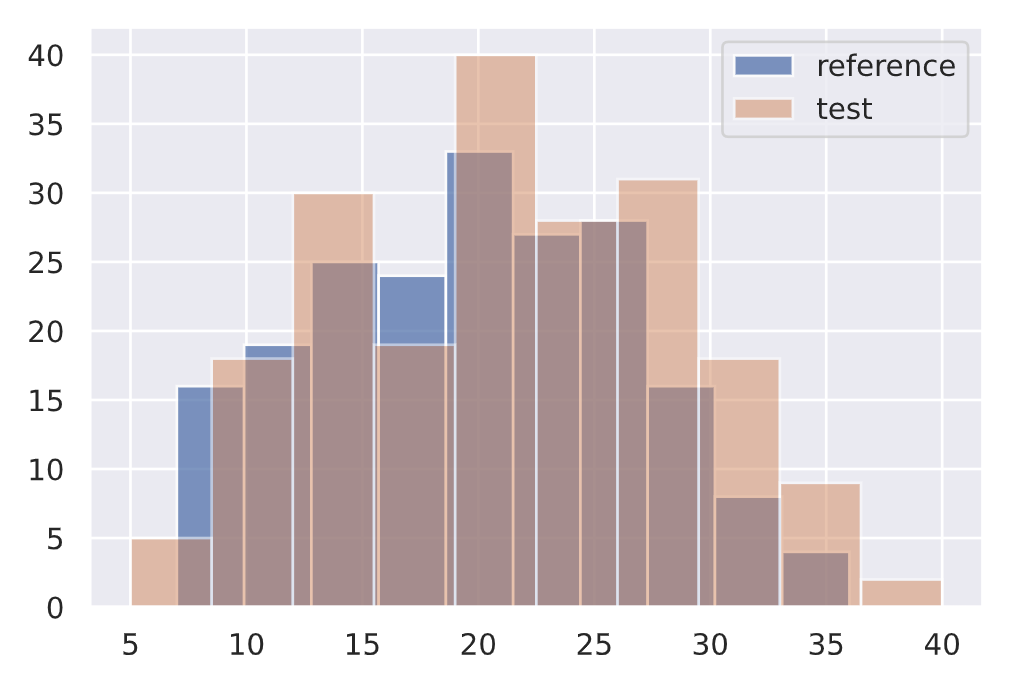
Our task may involve univariate (1D) features that we will want to monitor. While there are many types of hypothesis tests we can use, a popular option is the Kolmogorov-Smirnov (KS) test.
Kolmogorov-Smirnov (KS) test
The KS test determines the maximum distance between two distribution's cumulative density functions. Here, we'll measure if there is any drift on the size of our input text feature between two different data subsets.
Tip
While text is a direct feature in our task, we can also monitor other implicit features such as % of unknown tokens in text (need to maintain a training vocabulary), etc. While they may not be used for our machine learning model, they can be great indicators for detecting drift.
1 | |
1 2 3 4 5 6 | |
1 2 | |
1 2 3 4 5 6 | |
1 | |
{'data': {'distance': array([0.09], dtype=float32),
  'is_drift': 0,
  'p_val': array([0.3927307], dtype=float32),
  'threshold': 0.01},
 'meta': {'data_type': None,
  'detector_type': 'offline',
  'name': 'KSDrift',
  'version': '0.9.1'}}
↓ p-value = ↑ confident that the distributions are different.
1 2 3 4 5 6 | |
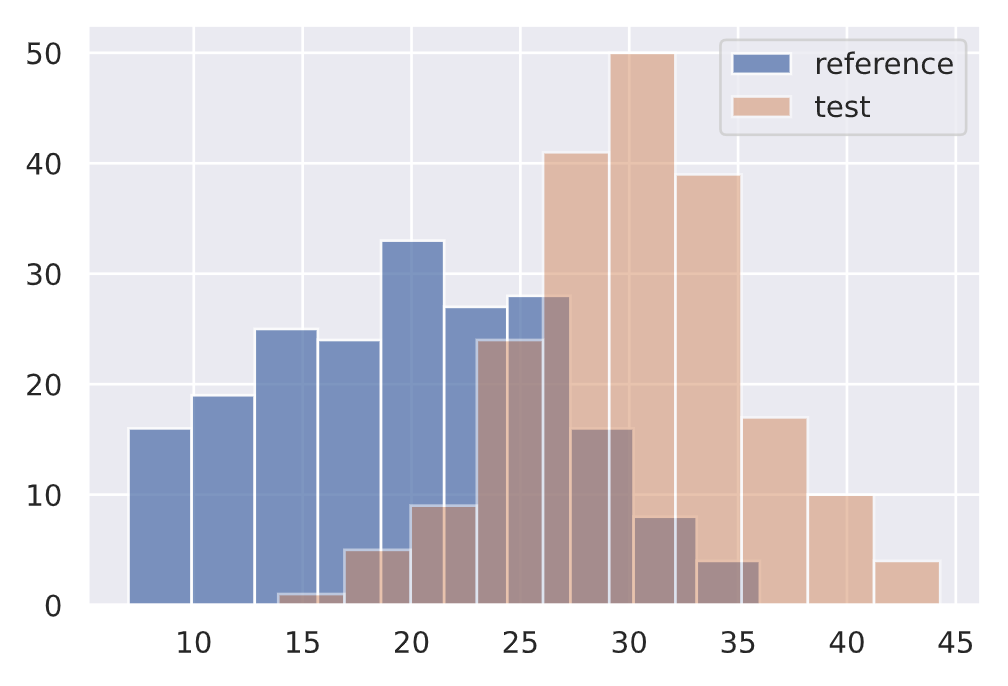
1 | |
{'data': {'distance': array([0.63], dtype=float32),
  'is_drift': 1,
  'p_val': array([6.7101775e-35], dtype=float32),
  'threshold': 0.01},
 'meta': {'data_type': None,
  'detector_type': 'offline',
  'name': 'KSDrift',
  'version': '0.9.1'}}
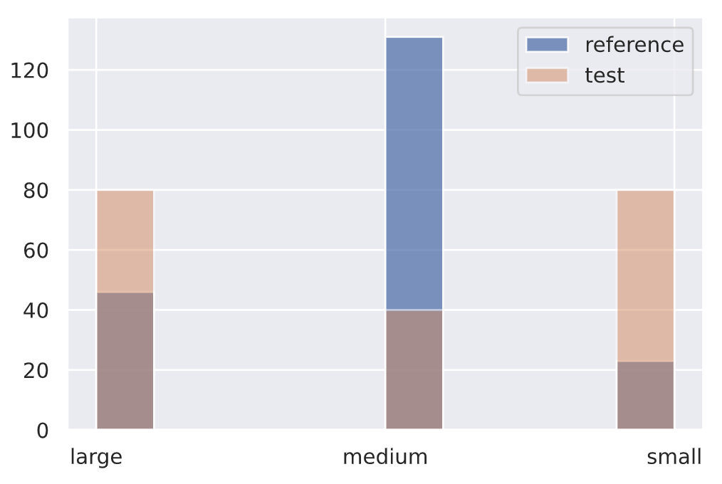
Chi-squared test
Similarly, for categorical data (input features, targets, etc.), we can apply the Pearson's chi-squared test to determine if a frequency of events in production is consistent with a reference distribution.
We're creating a categorical variable for the # of tokens in our text feature but we could very very apply it to the tag distribution itself, individual tags (binary), slices of tags, etc.
1 | |
1 2 3 4 5 | |
1 2 | |
1 2 3 4 5 6 | |
1 | |
{'data': {'distance': array([4.135522], dtype=float32),
  'is_drift': 0,
  'p_val': array([0.12646863], dtype=float32),
  'threshold': 0.01},
 'meta': {'data_type': None,
  'detector_type': 'offline',
  'name': 'ChiSquareDrift',
  'version': '0.9.1'}}
1 2 3 4 5 6 | |
1 | |
{'data': {'is_drift': 1,
  'distance': array([118.03355], dtype=float32),
  'p_val': array([2.3406739e-26], dtype=float32),
  'threshold': 0.01},
 'meta': {'name': 'ChiSquareDrift',
  'detector_type': 'offline',
  'data_type': None}}
Multivariate
As we can see, measuring drift is fairly straightforward for univariate data but difficult for multivariate data. We'll summarize the reduce and measure approach outlined in the following paper: Failing Loudly: An Empirical Study of Methods for Detecting Dataset Shift.
We vectorized our text using tf-idf (to keep modeling simple), which has high dimensionality and is not semantically rich in context. However, typically with text, word/char embeddings are used. So to illustrate what drift detection on multivariate data would look like, let's represent our text using pretrained embeddings.
Be sure to refer to our embeddings and transformers lessons to learn more about these topics. But note that detecting drift on multivariate text embeddings is still quite difficult so it's typically more common to use these methods applied to tabular features or images.
We'll start by loading the tokenizer from a pretrained model.
1 | |
1 2 3 4 | |
31090
1 2 3 4 | |
1 2 | |
tensor([  102,  2029,   467,  1778,   609,   137,  6446,  4857,   191,  1332,
         2399, 13572, 19125,  1983,   147,  1954,   165,  6240,   205,   185,
          300,  3717,  7434,  1262,   121,   537,   201,   137,  1040,   111,
          545,   121,  4714,   205,   103,     0,     0,     0,     0,     0,
            0,     0,     0,     0,     0,     0,     0,     0,     0,     0,
            0,     0,     0,     0,     0,     0,     0,     0,     0,     0,
            0])
[CLS] comparison between yolo and rcnn on real world videos bringing theory to experiment is cool. we can easily train models in colab and find the results in minutes. [SEP] [PAD] [PAD] ...
1 2 | |
['[CLS]', 'comparison', 'between', 'yo', '##lo', 'and', 'rc', '##nn', 'on', 'real', 'world', 'videos', 'bringing', 'theory', 'to', 'experiment', 'is', 'cool', '.', 'we', 'can', 'easily', 'train', 'models', 'in', 'col', '##ab', 'and', 'find', 'the', 'results', 'in', 'minutes', '.', '[SEP]', '[PAD]', '[PAD]', ...]
Next, we'll load the pretrained model's weights and use the TransformerEmbedding object to extract the embeddings from the hidden state (averaged across tokens).
1 | |
1 2 3 4 | |
1 2 3 | |
768
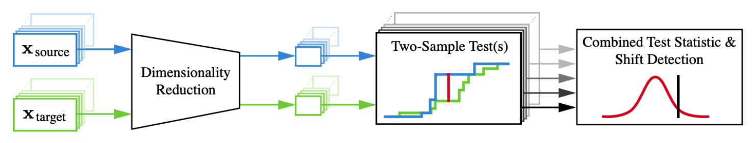
Dimensionality reduction
Now we need to use a dimensionality reduction method to reduce our representations dimensions into something more manageable (ex. 32 dim) so we can run our two-sample tests on to detect drift. Popular options include:
- Principle component analysis (PCA): orthogonal transformations that preserve the variability of the dataset.
- Autoencoders (AE): networks that consume the inputs and attempt to reconstruct it from an lower dimensional space while minimizing the error. These can either be trained or untrained (the Failing loudly paper recommends untrained).
- Black box shift detectors (BBSD): the actual model trained on the training data can be used as a dimensionality reducer. We can either use the softmax outputs (multivariate) or the actual predictions (univariate).
1 2 | |
1 2 3 | |
cuda
1 2 3 4 5 6 7 8 | |
We can wrap all of the operations above into one preprocessing function that will consume input text and produce the reduced representation.
1 2 | |
1 2 3 4 5 | |
Maximum Mean Discrepancy (MMD)
After applying dimensionality reduction techniques on our multivariate data, we can use different statistical tests to calculate drift. A popular option is Maximum Mean Discrepancy (MMD), a kernel-based approach that determines the distance between two distributions by computing the distance between the mean embeddings of the features from both distributions.
1 | |
1 2 | |
1 2 3 | |
{'data': {'distance': 0.0021169185638427734,
  'distance_threshold': 0.0032651424,
  'is_drift': 0,
  'p_val': 0.05999999865889549,
  'threshold': 0.01},
 'meta': {'backend': 'pytorch',
  'data_type': None,
  'detector_type': 'offline',
  'name': 'MMDDriftTorch',
  'version': '0.9.1'}}
1 2 3 | |
{'data': {'distance': 0.014705955982208252,
  'distance_threshold': 0.003908038,
  'is_drift': 1,
  'p_val': 0.0,
  'threshold': 0.01},
 'meta': {'backend': 'pytorch',
  'data_type': None,
  'detector_type': 'offline',
  'name': 'MMDDriftTorch',
  'version': '0.9.1'}}
Online
So far we've applied our drift detection methods on offline data to try and understand what reference window sizes should be, what p-values are appropriate, etc. However, we'll need to apply these methods in the online production setting so that we can catch drift as easy as possible.
Many monitoring libraries and platforms come with online equivalents for their detection methods.
Typically, reference windows are large so that we have a proper benchmark to compare our production data points to. As for the test window, the smaller it is, the more quickly we can catch sudden drift. Whereas, a larger test window will allow us to identify more subtle/gradual drift. So it's best to compose windows of different sizes to regularly monitor.
1 | |
1 2 3 4 | |
Generating permutations of kernel matrix..
100%|██████████| 1000/1000 [00:00<00:00, 13784.22it/s]
Computing thresholds: 100%|██████████| 200/200 [00:32<00:00,  6.11it/s]
As data starts to flow in, we can use the detector to predict drift at every point. Our detector should detect drift sooner in our drifter dataset than in our normal data.
1 2 3 4 5 6 7 8 9 10 11 | |
1 2 3 | |
27 steps
1 2 3 | |
11 steps
There are also several considerations around how often to refresh both the reference and test windows. We could base in on the number of new observations or time without drift, etc. We can also adjust the various thresholds (ERT, window size, etc.) based on what we learn about our system through monitoring.
Outliers
With drift, we're comparing a window of production data with reference data as opposed to looking at any one specific data point. While each individual point may not be an anomaly or outlier, the group of points may cause a drift. The easiest way to illustrate this is to imagine feeding our live model the same input data point repeatedly. The actual data point may not have anomalous features but feeding it repeatedly will cause the feature distribution to change and lead to drift.
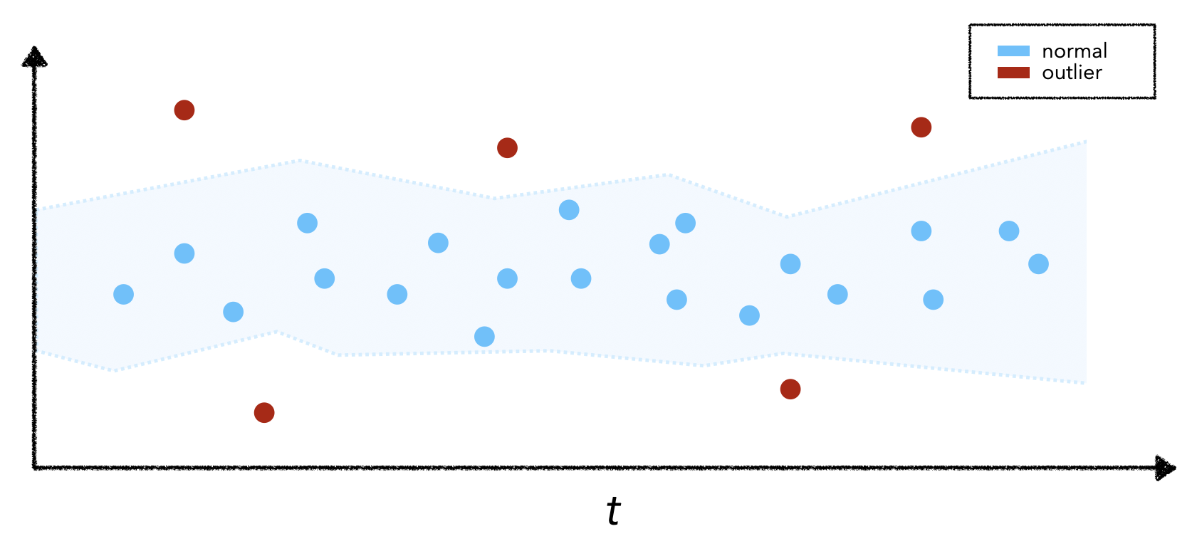
Unfortunately, it's not very easy to detect outliers because it's hard to constitute the criteria for an outlier. Therefore the outlier detection task is typically unsupervised and requires a stochastic streaming algorithm to identify potential outliers. Luckily, there are several powerful libraries such as PyOD, Alibi Detect, WhyLogs (uses Apache DataSketches), etc. that offer a suite of outlier detection functionality (largely for tabular and image data for now).
Typically, outlier detection algorithms fit (ex. via reconstruction) to the training set to understand what normal data looks like and then we can use a threshold to predict outliers. If we have a small labeled dataset with outliers, we can empirically choose our threshold but if not, we can choose some reasonable tolerance.
1 2 3 4 5 6 7 8 9 10 11 | |
When we identify outliers, we may want to let the end user know that the model's response may not be reliable. Additionally, we may want to remove the outliers from the next training set or further inspect them and upsample them in case they're early signs of what future distributions of incoming features will look like.
Solutions
It's not enough to just be able to measure drift or identify outliers but to also be able to act on it. We want to be able to alert on drift, inspect it and then act on it.
Alert
Once we've identified outliers and/or measured statistically significant drift, we need to a devise a workflow to notify stakeholders of the issues. A negative connotation with monitoring is fatigue stemming from false positive alerts. This can be mitigated by choosing the appropriate constraints (ex. alerting thresholds) based on what's important to our specific application. For example, thresholds could be:
- fixed values/range for situations where we're concretely aware of expected upper/lower bounds.
1
2
if percentage_unk_tokens > 5%: trigger_alert() - forecasted thresholds dependent on previous inputs, time, etc.
1
2
if current_f1 < forecast_f1(current_time): trigger_alert() - appropriate p-values for different drift detectors (↓ p-value = ↑ confident that the distributions are different).
1
2
from alibi_detect.cd import KSDrift
length_drift_detector = KSDrift(reference, p_val=0.01)
Once we have our carefully crafted alerting workflows in place, we can notify stakeholders as issues arise via email, Slack, PageDuty, etc. The stakeholders can be of various levels (core engineers, managers, etc.) and they can subscribe to the alerts that are relevant for them.
Inspect
Once we receive an alert, we need to inspect it before acting on it. An alert needs several components in order for us to completely inspect it:
- specific alert that was triggered
- relevant metadata (time, inputs, outputs, etc.)
- thresholds / expectations that failed
- drift detection tests that were conducted
- data from reference and test windows
- log records from the relevant window of time
# Sample alerting ticket
{
    "triggered_alerts": ["text_length_drift"],
    "threshold": 0.05,
    "measurement": "KSDrift",
    "distance": 0.86,
    "p_val": 0.03,
    "reference": [],
    "target": [],
    "logs": ...
}
With these pieces of information, we can work backwards from the alert towards identifying the root cause of the issue. Root cause analysis (RCA) is an important first step when it comes to monitoring because we want to prevent the same issue from impacting our system again. Often times, many alerts are triggered but they maybe all actually be caused by the same underlying issue. In this case, we'd want to intelligently trigger just one alert that pinpoints the core issue. For example, let's say we receive an alert that our overall user satisfaction ratings are reducing but we also receive another alert that our North American users also have low satisfaction ratings. Here's the system would automatically assess for drift in user satisfaction ratings across many different slices and aggregations to discover that only users in a specific area are experiencing the issue but because it's a popular user base, it ends up triggering all aggregate downstream alerts as well!
Act
There are many different ways we can act to drift based on the situation. An initial impulse may be to retrain our model on the new data but it may not always solve the underlying issue.
- ensure all data expectations have passed.
- confirm no data schema changes.
- retrain the model on the new shifted dataset.
- move the reference window to more recent data or give it more weight.
- determine if outliers are potentially valid data points.
Production
Since detecting drift and outliers can involve compute intensive operations, we need a solution that can execute serverless workloads on top of our event data streams (ex. Kafka). Typically these solutions will ingest payloads (ex. model's inputs and outputs) and can trigger monitoring workloads. This allows us to segregate the resources for monitoring from our actual ML application and scale them as needed.
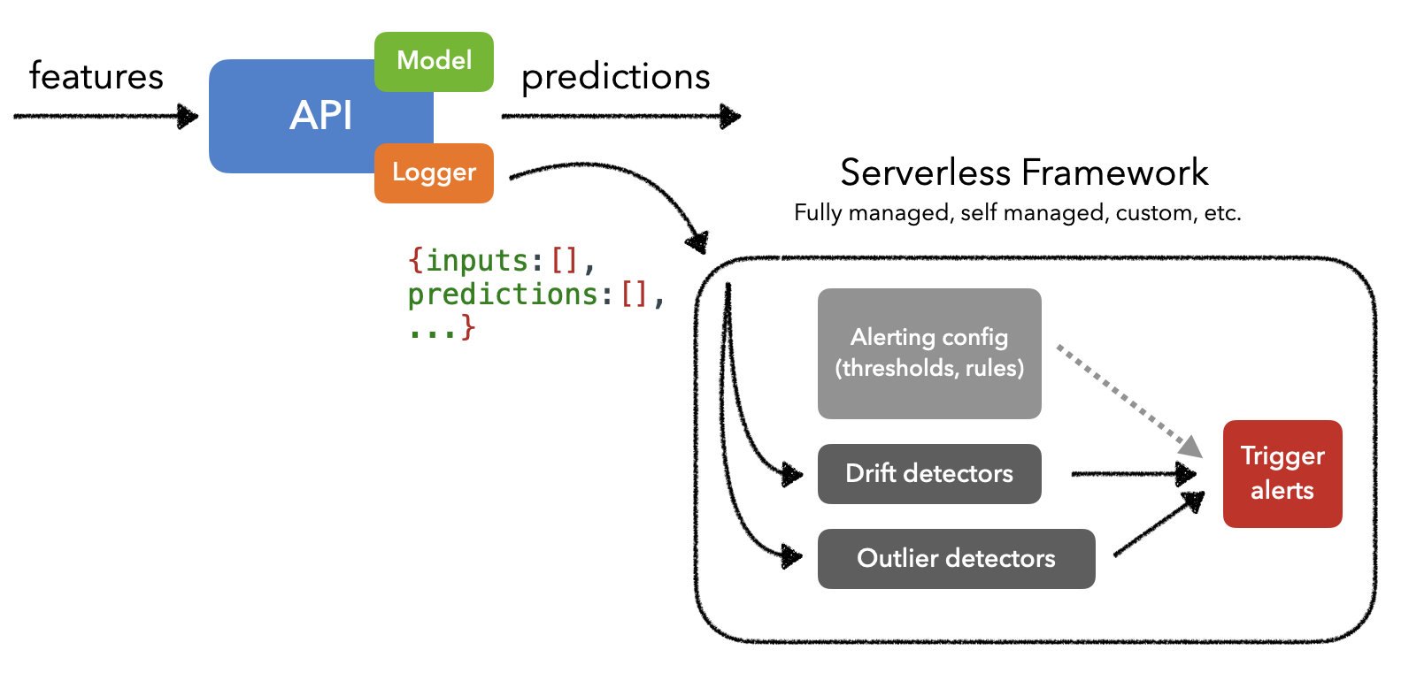
When it actually comes to implementing a monitoring system, we have several options, ranging from fully managed to from-scratch. Several popular managed solutions are Arize, Arthur, Fiddler, Gantry, Mona, WhyLabs, etc., all of which allow us to create custom monitoring views, trigger alerts, etc. There are even several great open-source solutions such as EvidentlyAI, TorchDrift, WhyLogs, etc.
We'll often notice that monitoring solutions are offered as part of the larger deployment option such as Sagemaker, TensorFlow Extended (TFX), TorchServe, etc. And if we're already working with Kubernetes, we could use KNative or Kubeless for serverless workload management. But we could also use a higher level framework such as KFServing or Seldon core that natively use a serverless framework like KNative.
References
- An overview of unsupervised drift detection methods
- Failing Loudly: An Empirical Study of Methods for Detecting Dataset Shift
- Monitoring and explainability of models in production
- Detecting and Correcting for Label Shift with Black Box Predictors
- Outlier and anomaly pattern detection on data streams
Upcoming live cohorts
Sign up for our upcoming live cohort, where we'll provide live lessons + QA, compute (GPUs) and community to learn everything in one day.
To cite this content, please use:
1 2 3 4 5 6 | |